A Least Squares Approach

---

The essentials

Choose w to get the min Loss function.

$\mathcal { L } = \frac { 1 } { N } \sum _ { n = 1 } ^ { N } \mathcal { L } _ { n } \left( t _ { n } , f \left( x _ { n } ; \vec{w} \right) \right)$ $\underset { \vec{w} } { \operatorname { argmin } } \frac { 1 } { N } \sum _ { n = 1 } ^ { N } \mathcal { L } _ { n } \left( t _ { n } , f \left( x _ { n } ; \vec{w} \right) \right)$ we can change $\mathcal { L } _ { n }$ to fit our needs, but here we use the mostly used square root sum function.
$\mathcal { L } _ { n } \left( t _ { n } , f \left( x _ { n } ; w _ { 0 } , w _ { 1 } \right) \right) = \left( t _ { n } - f \left( x _ { n } ; w _ { 0 } , w _ { 1 } \right) \right) ^ { 2 }$

Turning point

Goal: to choose the minimum in a mathmatical way. How it works: the partial derivatives of $\mathbf{w}$ should be $0$, and second derivatives should be a positive value to ensure this is a minimum/maxmum

Example

$\mathbf{w} =\left[ \begin{array} { l } { w _ { 0 } } \\ { w _ { 1 } } \end{array} \right] \Rightarrow \begin{cases} & \widehat { w _ { 0 } } = \overline { t } - w _ { 1 } \overline { x }\\ & \widehat { w _ { 1 } } = \frac { \overline { x t } - \overline { x } \overline { t } } { x ^ { 2 } - ( \overline { x } ) ^ { 2 } } \end{cases}$

#data.csv
n xn tn xntn x2
1 1896 12.00 22752.0 3.5948*10**6
2 1900 11.00 20900.0 3.6100*10**6
3 1904 11.00 20944.0 3.6252*10**6
4 1906 11.20 21347.2 3.6328*10**6
5 1908 10.80 20606.4 3.6405*10**6
6 1912 10.80 20649.6 3.6557*10**6
7 1920 10.80 20736.0 3.6864*10**6
8 1924 10.60 20394.4 3.7018*10**6
9 1928 10.80 20822.4 3.7172*10**6
10 1932 10.30 19899.6 3.7326*10**6
11 1936 10.30 19940.8 3.7481*10**6
12 1948 10.30 20064.4 3.7947*10**6
13 1952 10.40 20300.8 3.8103*10**6
14 1956 10.50 20538.0 3.8259*10**6
15 1960 10.20 19992.0 3.8416*10**6
16 1964 10.00 19640.0 3.8573*10**6
17 1968 9.95 19581.6 3.8730*10**6
18 1972 10.14 19996.1 3.8888*10**6
19 1976 10.06 19878.6 3.9046*10**6
20 1980 10.25 20295.0 3.9204*10**6
21 1984 9.99 19820.2 3.9363*10**6
22 1988 9.92 19721.0 3.9521*10**6
23 1992 9.96 19840.3 3.9681*10**6
24 1996 9.84 19640.6 3.9840*10**6
25 2000 9.87 19740.0 4.0000*10**6
26 2004 9.85 19739.4 4.0160*10**6
27 2008 9.69 19457.5 4.0321*10**6

# python3
import numpy as np
import pandas as pd
import copy as copy
import matplotlib.pyplot as plt

df = pd.read_csv('data.csv',sep=' ')
mm = copy.deepcopy(df)
for index, row in df.iterrows():
    df.loc[index,'x2'] =  eval(df.iloc[index]['x2'])
    print(int(df.iloc[index]['x2']))

mean = df.mean()
w1 = (mean['xntn']-mean['xn']*mean['tn'])/(mean['x2'] -mean['xn']*mean['xn'])
w0 = mean['tn'] - w1*mean['xn']
xn = mm.loc[:,'xn']
tn = mm.loc[:,'tn']
x = np.linspace(1870,2020,100) # 100 linearly spaced numbers
y = w0 + w1*x
plt.xlabel('Years', fontsize = 30)
plt.ylabel('Time(second)', fontsize = 30)
plt.plot(xn, tn, 'ro')
plt.plot(x,y)
plt.show()

Result:

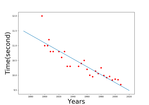$f \left( x ; w _ { 0 } , w _ { 1 } \right) = 36.416 - 0.013 x$ Linear model

Vector/ Matrix notation

why?

• To express many variables in one time example:
• $f \left( x _ { n } ; w _ { 0 } , w _ { 1 } \right) = \mathbf { w } ^ { \top } \mathbf { x } _ { n } = w _ { 0 } + w _ { 1 } x _ { n }$
• $\mathcal { L } = \frac { 1 } { N } ( \mathbf { t } - \mathbf { X w } ) ^ { \top } ( \mathbf { t } - \mathbf { X } \mathbf { w } )$
• $\mathbf { X } = \left[ \begin{array} { c } { \mathbf { x } _ { 1 } ^ { \top } } \\ { \mathbf { x } _ { 2 } ^ { \top } } \\ { \vdots } \\ { \mathbf { x } _ { N } ^ { \top } } \end{array} \right] = \left[ \begin{array} { c c } { 1 } & { x _ { 1 } } \\ { 1 } & { x _ { 2 } } \\ { \vdots } & { \vdots } \\ { 1 } & { x _ { N } } \end{array} \right] , \quad \mathbf { t } = \left[ \begin{array} { c } { t _ { 1 } } \\ { t _ { 2 } } \\ { \vdots } \\ { t _ { N } } \end{array} \right]$
• $\mathbf { w } = \left[ \begin{array} { c } { w _ { 0 } } \\ { w _ { 1 } } \end{array} \right] , \quad \mathbf { x } _ { n } = \left[ \begin{array} { c } { 1 } \\ { x _ { n } } \end{array} \right]$
• $\frac { \partial \mathcal { L } } { \partial \mathbf { w } } = \left[ \begin{array} { l } { \frac { \partial \mathcal { L } } { \partial w _ { 0 } } } \\ { \frac { \partial \mathcal { L } } { \partial w _ { 1 } } } \end{array} \right]$

useful identities: $\begin{array} { c | c } f ( \mathbf { w } ) & \quad \frac { \partial f } { \partial \mathbf { w } }\\{ \mathbf { w } ^ { \top } \mathbf { x } } & { \mathbf { x } }\\{ \mathbf { x } ^ { \top } \mathbf { w } } & { \mathbf { x } } \\ { \mathbf { w } ^ { \top } \mathbf { w } } & { 2 \mathbf { w } } \\ { \mathbf { w } ^ { \top } \mathbf { C } \mathbf { w } } & { 2 \mathbf { C } \mathbf { w } } \end{array}$

Squre root

$\widehat { \mathbf { w } } = \left( \mathbf { X } ^ { \top } \mathbf { X } \right) ^ { - 1 } \mathbf { X } ^ { \top } \mathbf { t }$

# data is the same as above
import numpy as np
import pandas as pd
import copy as copy
import matplotlib.pyplot as plt

df = pd.read_csv('data.csv',sep=' ')
mm = copy.deepcopy(df)
for index, row in df.iterrows():
    df.loc[index,'x2'] =  eval(df.iloc[index]['x2'])
    #print(int(df.iloc[index]['x2']))

mean = df.mean()
X = np.ones(mm.shape[0]*2).reshape(mm.shape[0],2)
t = np.ones(mm.shape[0]).reshape(mm.shape[0],1)
for index in range(X.shape[0]):
    X[index][1] = mm.loc[index, 'xn']
    t[index][0] = mm.loc[index, 'tn']
Xt = np.transpose(X)
w = np.dot(np.dot(np.linalg.inv(np.dot(Xt, X)) , Xt),t)
xn = mm.loc[:,'xn']
tn = mm.loc[:,'tn']
x = np.linspace(1870,2020,100) 
y = w[0] + w[1]*x
plt.xlabel('Years', fontsize = 30)
plt.ylabel('Time(second)', fontsize = 30)
plt.plot(xn, tn, 'ro')
plt.plot(x,y)
plt.show()

# print(w)
# out: array([[3.64164559e+01],[-1.33308857e-02]])
# the same result with above

# another better method and poly
import pylab as plt
import urllib.request
# You only need this line if you haven't cloned the repo...if you have cloned, you'll already have the data
urllib.request.urlretrieve('https://raw.githubusercontent.com/sdrogers/fcmlcode/master/notebooks/data/olympic100m.txt', 'olympic100m.txt')
import numpy as np
# If you have cloned, make sure this is pointing to the correct file, maybe ../data/olympic100m.txt ?
data = np.loadtxt('olympic100m.txt',delimiter=',')
x = data[:,0][:,None]
t = data[:,1][:,None]


X = np.hstack((np.ones_like(x),x,x**2))  # we just add more to here to change all 
X = np.asmatrix(X)
t = t # This is already a vector!

w = (X.T*X).I*X.T*t
testx = np.linspace(1896,2012,100)[:,None]
testX = np.hstack((np.ones_like(testx),testx,testx**2))
testt = testX*w
plt.figure()
plt.plot(x,t,'ro')
plt.plot(testx,testt,'b')
plt.show()

…

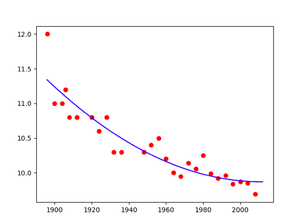Poly = 2 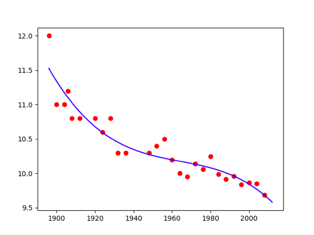Poly = 3

we are free to define any set of K functions of X $\mathbf { X } = \left[ \begin{array} { c c c c } { h _ { 1 } \left( x _ { 1 } \right) } & { h _ { 2 } \left( x _ { 1 } \right) } & { \cdots } & { h _ { K } \left( x _ { 1 } \right) } \\ { h _ { 1 } \left( x _ { 2 } \right) } & { h _ { 2 } \left( x _ { 2 } \right) } & { \cdots } & { h _ { K } \left( x _ { 2 } \right) } \\ { \vdots } & { \vdots } & { \cdots } & { \vdots } \\ { h _ { 1 } \left( x _ { N } \right) } & { h _ { 2 } \left( x _ { N } \right) } & { \cdots } & { h _ { K } \left( x _ { N } \right) } \end{array} \right]$

Like:

import pylab as plt
import urllib.request
# You only need this line if you haven't cloned the repo...if you have cloned, you'll already have the data
urllib.request.urlretrieve('https://raw.githubusercontent.com/sdrogers/fcmlcode/master/notebooks/data/olympic100m.txt', 'olympic100m.txt')
import numpy as np
import math
# If you have cloned, make sure this is pointing to the correct file, maybe ../data/olympic100m.txt ?
data = np.loadtxt('olympic100m.txt',delimiter=',')
x = data[:,0][:,None]
t = data[:,1][:,None]
hx = np.sin((x-2660)/4.3)

X = np.hstack((np.ones_like(x),x,hx))  # we just add more to here to change all 
X = np.asmatrix(X)
t = t # This is already a vector!

w = (X.T*X).I*X.T*t
testx = np.linspace(1896,2012,100)[:,None]
testX = np.hstack((np.ones_like(testx),testx,np.sin((testx-2660)/4.3)))
testt = testX*w
plt.figure()
plt.plot(x,t,'ro')
plt.plot(testx,testt,'b')
plt.show()

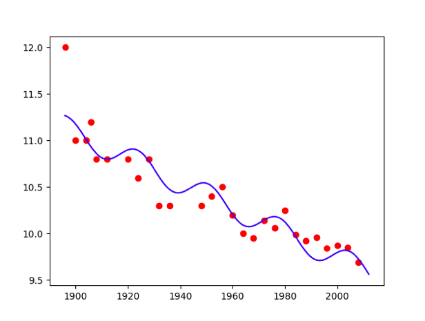… Polynomial model

Validation data

1. Why we need to validate?
   • to restrain overfitting
2. How we validate data?
   • a effecient technique – Cross-validation(K-fold)
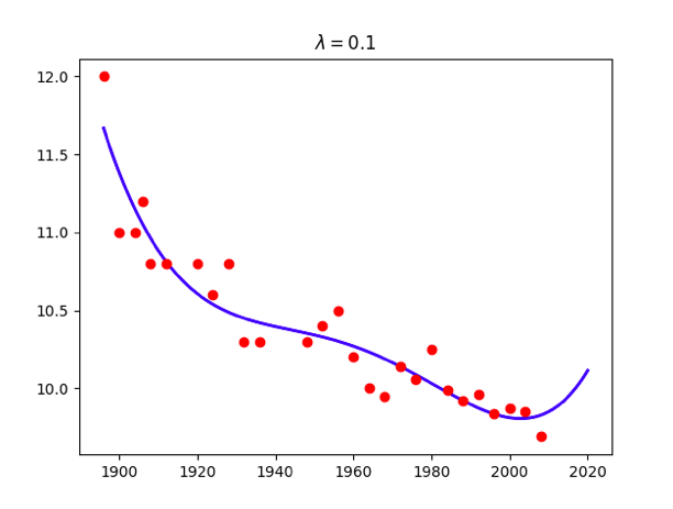
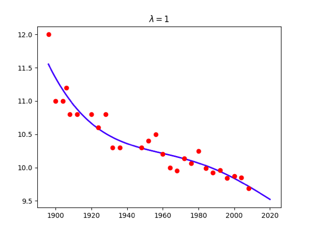
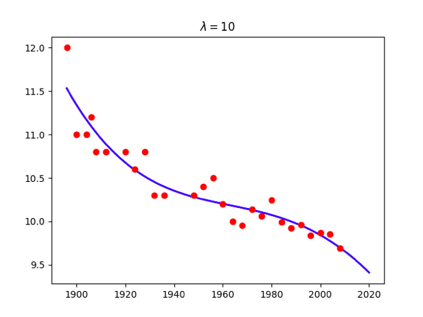
3. How to prevent from overfitting?
   • regularisation- if we don’t want our model to become too complex
     • $\mathcal { L } ^ { \prime } = \mathcal { L } + \lambda \mathbf { w } ^ { \top } \mathbf { w }$
     • $\widehat { \mathbf { w } } = \left( \mathbf { X } ^ { \top } \mathbf { X } + N \lambda \mathbf { I } \right) ^ { - 1 } \mathbf { X } ^ { \top } \mathbf { t }$

import pylab as plt
import urllib.request
# You only need this line if you haven't cloned the repo...if you have cloned, you'll already have the data
urllib.request.urlretrieve('https://raw.githubusercontent.com/sdrogers/fcmlcode/master/notebooks/data/olympic100m.txt', 'olympic100m.txt')
import numpy as np
import math
# If you have cloned, make sure this is pointing to the correct file, maybe ../data/olympic100m.txt ?
data = np.loadtxt('olympic100m.txt',delimiter=',')
x = data[:,0][:,None]
t = data[:,1][:,None]
maxorder = 7
x_test = np.linspace(1896,2020,100)[:,None]
X = np.ones_like(x)
X_test = np.ones_like(x_test)
for i in range(1,maxorder+1):
    X = np.hstack((X,x**i))
    X_test = np.hstack((X_test,x_test**i))

X = np.asmatrix(X)
for lamb in [0,0.01,0.1,1,10,100]:
    w = np.linalg.solve(np.dot(X.T,X) + x.size*lamb*np.identity(maxorder+1),np.dot(X.T,t))
    A = np.dot(X.T,X) 
   
    B = np.dot(X.T,t)
    m = A.I*B
    #w = np.linalg.solve(A,B)
    f_test = np.dot(X_test,w)
    plt.figure()
    plt.plot(x_test,f_test,'b-',linewidth=2)
    plt.plot(x,t,'ro')
    title = '<span class="katex"><span class="katex-mathml"><math xmlns="http://www.w3.org/1998/Math/MathML"><semantics><mrow><mi>λ</mi><mo>=</mo></mrow><annotation encoding="application/x-tex">\lambda=</annotation></semantics></math></span><span class="katex-html" aria-hidden="true"><span class="base"><span class="strut" style="height:0.69444em;vertical-align:0em;"></span><span class="mord mathdefault">λ</span><span class="mspace" style="margin-right:0.2777777777777778em;"></span><span class="mrel">=</span></span></span></span>%g'%lamb
    plt.title(title)

$lambda = 0.01$ $lambda = 0.1$ $lambda = 1$ $lambda = 10$

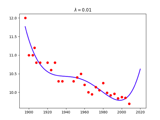
Attention: use np.linalg.solve(A,B) instead of $w = A ^ { - 1 }*B$ becauese the accuracy problem.

Cross-validation

The loss that we calculate from validation data will be sensitive to the choice of data in our validation set, especially dataset is small. so we need a method to make more efficient use of the data we have K-fold cross-validation, particularly, Leave-One-Out Cross-Validation(LOOCV) $\mathcal { L } ^ { C V } = \frac { 1 } { N } \sum _ { n = 1 } ^ { N } \left( t _ { n } - \widehat { \mathbf { w } } _ { - n } ^ { \top } \mathbf { x } _ { n } \right) ^ { 2 }$

The best model – minimize test loss

import pylab as plt
import urllib.request
# You only need this line if you haven't cloned the repo...if you have cloned, you'll already have the data
urllib.request.urlretrieve('https://raw.githubusercontent.com/sdrogers/fcmlcode/master/notebooks/data/olympic100m.txt', 'olympic100m.txt')
import numpy as np
import math
# If you have cloned, make sure this is pointing to the correct file, maybe ../data/olympic100m.txt ?
data = np.loadtxt('olympic100m.txt',delimiter=',')
x = data[:,0][:,None]
t = data[:,1][:,None]
maxorder = 8
x_train = x[:-3]
x_test = x[-3:]
t_train = t[:-3]
t_test = t[-3:]
X_train = np.ones_like(x_train)
X_test = np.ones_like(x_test)
errorlist = []
errorstdlist = []
for i in range(1,maxorder+1):
    X_train = np.hstack((X_train,x_train**i))
    X_test = np.hstack((X_test,x_test**i))
    w = np.linalg.solve(np.dot(X_train.T,X_train) ,np.dot(X_train.T,t_train))
    #w = np.linalg.solve(A,B)
    f_test = np.dot(X_test,w)
    error_std = np.std(f_test - t_test)
    errorstdlist.append(np.std(np.dot(X_train,w) - t_train))
    errorlist.append (error_std)
    f_test = np.dot(X_test,w)
plt.figure()
plt.plot([1,2,3,4,5,6,7,8],errorlist,'b-',linewidth=2)
plt.plot([1,2,3,4,5,6,7,8],errorstdlist,'y-',linewidth=2)
plt.show()

Best model visualization Then we can choose the best model.

LOOCV loss and train, test less

LOOCV loss: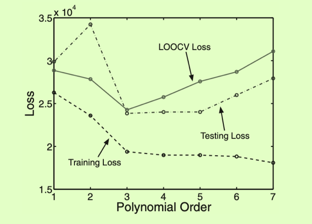

---

You May Also Enjoy

How To Train Multiple Model In One Time With Sklearn --Machine Learning

Linear Modeling - A Maximum Likelihood Approach --Machine Learning --Math

The Bayesian Approach To Machine Learning --Machine Learning --Math

An Introduction To ESN --Math

Modeling With NMF And SVD --Machine Learning --Math

Feature Engineering For Machine Learning --Machine Learning

Welcome to share or comment on this post: