2019 August 20 Machine Learning, Math

Bounding Box Regression

What is bounding box regression?

Find a $f$ to map the raw input window $P$ to real window $G$ , we get $\hat { { G } }$ . $f(P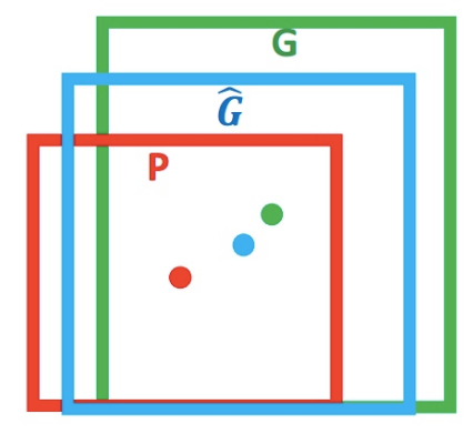) = \hat { { G } }, \hat { { G } } \approx G$ Figure 1

Why we need it?

To learn a transformation that maps a proposed box $P$ to a ground-truth box $G$ . You know, if we don’t define something to optimize, we cannot achive the goals. 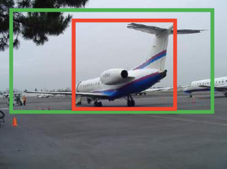Figure 2

What is IoU(Intersection over Union)?

Notice the green and red box below. 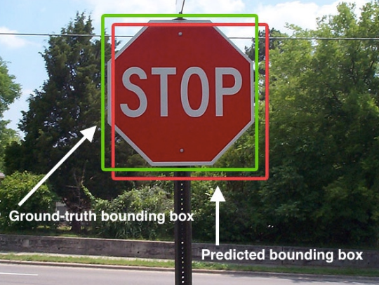Figure 3

We use Bounding Box Regression to adjust that red window to approach green window. 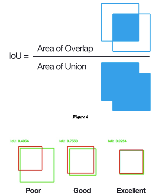Figure 4

## get IoU according to box parameters
# import the necessary packages
from collections import namedtuple
import numpy as np
import cv2

# define the `Detection` object
Detection = namedtuple("Detection", ["image_path", "gt", "pred"])

def bb_intersection_over_union(boxA, boxB):
    # determine the (x, y)-coordinates of the intersection rectangle
    xA = max(boxA[0], boxB[0])
    yA = max(boxA[1], boxB[1])
    xB = min(boxA[2], boxB[2])
    yB = min(boxA[3], boxB[3])

    # compute the area of intersection rectangle
    interArea = (xB - xA) * (yB - yA)

    # compute the area of both the prediction and ground-truth
    # rectangles
    boxAArea = (boxA[2] - boxA[0]) * (boxA[3] - boxA[1])
    boxBArea = (boxB[2] - boxB[0]) * (boxB[3] - boxB[1])

    # compute the intersection over union by taking the intersection
    # area and dividing it by the sum of prediction + ground-truth
    # areas - the interesection area
    iou = interArea / float(boxAArea + boxBArea - interArea)

    # return the intersection over union value
    return iou

You see, it’s easy to calculate IOU using python.

How we find that function $\hat{G}$ ?

Target mapping $f$ :

$\left( P _{ x } , P_ { y } , P _{ w } , P_ { h } \right) = \left( \hat { G } _{ x } , \hat { G }_ { y } , \hat { G } _{ w } , \hat { G }_ { h } \right) ,\left( \hat { G } _{ x } , \hat { G }_ { y } , \hat { G } _{ w } , \hat { G }_ { h } \right) \approx \left( G _{ x } , G_ { y } , G _{ w } , G_ { h } \right)$

How to map $P$ to $\hat { G }$ in figure 1?

Core concept

translation
- $( \Delta x , \Delta y ) , \quad \Delta x = P _{ w } d_ { x } ( P ) , \Delta y = P _{ h } d_ { y } ( P )$ $\begin{aligned} \hat { G } _{ x } = P_ { w } d _{ x } ( P ) + P_ { x } \\ \hat { G } _{ y } = P_ { h } d _{ y}( P ) + P_ { y } \tag{1} \end{aligned}$
scaling
- $\left( S _{ w } , S_ { h } \right) , S _{ w } = \exp \left( d_ { w } ( P ) \right) , S _{ h } = \exp \left( d_ { h } ( P ) \right)$ $\begin{aligned} \hat { G } _{ w } & = P_ { w } \exp \left( d _{ w } ( P ) \right) \\ \hat { G }_ { h } & = P _{ h } \exp \left( d_ { h } ( P ) \right) \tag{2} \end{aligned}$
  That means, bounding box regression is to learning $d _{ x } ( P ) , d_ { y } ( P ) , d _{ w } ( P ) , d_ { h } ( P )$ , we can find that we could use $d _{ *} ( P ) = \mathbf { w }_{ \star } ^ { \mathrm { T } } \phi _{ 5 } ( P )$ to learn how to map $\phi_ {5}$ (pool5 features of proposal P) to $d _{*}$ , which is a simple linear regression problem, and we can use the formula $(1)$ - $(2)$ to get $\hat {G}$ .

$\hat { { G } }$ is forecast value, but we need $\hat { { G } }$ to be $G$ . So we still need to find the difference between $G$ and $\hat { { G } }$ .

What’s the difference between $\hat { { G } }$ and $G$ ?

We want $\hat { { G } }$ to be as close to $G$ as possible, that means, we need to find a bounding box input: features of proposal $\phi _{5}$ (CNN pool5 output) bounding box output: $d _{ x } ( P ) , d_ { y } ( P ) , d _{ w } ( P ) , d_ { h } ( P )$ . Then we can map $P$ to $G$ .

How to use the bounding box output to get $G$ ?

From above we can know that we could get $\hat { { G } }$ from $d _{ x } ( P ) , d_ { y } ( P ) , d _{ w } ( P ) , d_ { h } ( P )$ , not $G$ . Notice, from $P$ to $G$ means: $\begin{aligned} t _{ x } = \left( G_ { x } - P _{ x } \right) / P_ { w } \\ t _{ y } = \left( G_ { y } - P _{ y } \right) / P_ { h }\\ t _{ w } = \log \left( G_ { w } / P _ { w } \right) \\ t _{ h } = \log \left( G_ { h } / P _ { h } \right) \end{aligned}$

That means if we reduce the error between $d _{ x } ( P ) , d_ { y } ( P ) , d _{ w } ( P ) , d_ { h } ( P )$ and $t _{ *} = \left( t*_ *{ x } , t _{ y } , t_ { w } , t _{ h } \right) )$ , we can really map our $P$ to $G$ , because we have bounding box help use to learn the real $t_ {*}$ for us. $\Rightarrow$
We can reduce the loss function: $L o s s = \sum _{ i } ^ { N } \left( t_ { * } ^ { i } - W ^ { T } \phi _ { 5 } \left( P ^ { i } \right) \right) ^ { 2 }$ to accomplish our goal. Here $\phi _ { 5 } \left( P ^ { i } \right)$ means the input to bounding box.

Also to regularize the loss function, we can use: $W _{ * } = \operatorname { argmin }_ { w , } \sum _{ i } ^ { N } \left( t_ { * } ^ { i } - W ^ { T } \phi _{ 5 } \left( P ^ { i } \right) \right) ^ { 2 } + \lambda \left\| \hat { w }_ { * } \right\| ^ { 2 }$ and use gredient descent to get $W$ .

Why we can use $\hat { G } = WP$ ?

When IoU > $\theta$ (like 0.6), we can think the transformation be a linear transformation, and use that function to adjust. $t _{ w } = \log \left( G_ { w } / P _{ w } \right) = \log \left( \frac { G_ { w } + P _{ w } - P_ { w } } { P _{ w } } \right) = \log \left( 1 + \frac { G_ { w } - P _{ w } } { P_ { w } } \right)$ When $G _{ w } - P_ { w } \approx 0$ , we think it as linear. $\lim _ { x = 0 } \log ( 1 + x ) = x$

Bounding Box Regression