Linear Modeling - A Maximum Likelihood Approach | Blog
2019 September 06Machine Learning, Math
Linear Modeling - A Maximum Likelihood Approach
ERRORS AS NOISE
Explicitly model the noise (the errors between the model and the observations) in the data by incorporating a random variable.
Advantages of incorporating a noise term into our model:
Allows us to express the level of uncertainty in our estimate of the model parameters, w
Provides several benefits over loss minimisation.
Able to quantify the uncertainty in our parameters and the ability to express uncertainties in our predictions(just use the available).
How to present linear model that fit our data
For linear model, we can add a variable to think in a generative way. tn=wTxn+ϵnϵn is continuous random variable
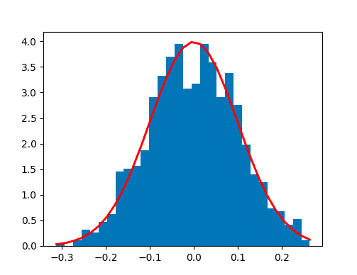
also, ϵn should be independent, which means: p(ϵ1,…,ϵN)=∏n=1Np(ϵn). Usually, we use gaussian distribution: p(ϵ)=N(μ,σ2)
mu,sigma=0,0.1# mean and standard deviation
s=np.random.normal(mu,sigma,1000)print(abs(mu-np.mean(s))<0.01)print(abs(sigma-np.std(s,ddof=1))<0.01)importmatplotlib.pyplotaspltcount,bins,ignored=plt.hist(s,30,density=True)plt.plot(bins,1/(sigma*np.sqrt(2*np.pi))*np.exp(-(bins-mu)**2/(2*sigma**2)),linewidth=2,color='r')plt.show()##out
#true
#true
Guassian Distribution
importnumpyasnpmu,sigma=0,0.05# mean and standard deviation
s=np.random.normal(mu,sigma,10)x=np.vstack(np.linspace(0,9,num=10))w=np.array([-0.05,9.375])xx=np.hstack((x,np.ones_like(x)))y=xx@w+splt.scatter(x.T,y)plt.show()
Linear sample
Dataset likelihood
Usually we are not interested in the likelihood of a single data point but that of all of the data, like:
p(t1,…,tN∣x1,…,xN,w,σ2) for short p(t∣X,w,σ2)
We assume p is gaussian distribution, and noise at each point is completely independent, then L=p(t∣X,w,σ2)=∏n=1Np(tn∣xn,w,σ2)=∏n=1NN(w⊤xn,σ2) (*)
tn are conditionally independent – given a value for w, the tn are independent Eg: To get p(t1960∣x1960,X,t)
we can have p(t1960∣x1960,X,t)=p(t∣X)p(t1960,t∣x1960,X)
that shows in our model, tn are conditionally independent – given a value for w, the tn are independent. This dependence is encapsulated in the parameter w. In a word, if we know w, all that remains is the errors between the observed data and wTxn, errors are independent(noise–gaussian distribution),conditioned on w, the observations are independent. Without a model (and therefore a w), the observations are not independent.
Maximum likelihood
Why we need to maximum the likelihood?
Because we have a fixed dataset, varying the model will result in different likelihood values, so a sensible choice of model would be that which maximised the likelihood ==> choose the w and σ2 to maximum L.
∑n=1Nxntn can be write as XTt and ∑n=1Nxnxn⊤w can be write as XTXw then\
∂w∂logL=σ21(X⊤t−X⊤Xw)=0⇒w=(X⊤X)−1X⊤t the same as the result we got in the previous chapter.
Also for σ ∂σ∂logL=−σN+σ31∑n=1N(tn−x⊤w)2=0 σ2=N1(t−Xw)⊤(t−Xw)=N1(t⊤t−2t⊤Xw+w⊤X⊤Xw) σ2=N1(t⊤t−2t⊤X(X⊤X)−1X⊤t+t⊤X(X⊤X)−1X⊤X(X⊤X)−1X⊤t)=N1(t⊤t−2t⊤X(X⊤X)−1X⊤t+t⊤X(X⊤X)−1X⊤t)=N1(t⊤t−t⊤X(X⊤X)−1X⊤t)
importpylabaspltimporturllib.requesturllib.request.urlretrieve('https://raw.githubusercontent.com/sdrogers/fcmlcode/master/notebooks/data/olympic100m.txt','olympic100m.txt')importnumpyasnpimportmathdata=np.loadtxt('olympic100m.txt',delimiter=',')x=data[:,0][:,None]t=data[:,1][:,None]X=np.hstack((np.ones_like(x),x))# we just add more to here to change all
X=np.asmatrix(X)t=t# This is already a vector!
w=(X.T*X).I*X.T*tdelta=(1.0/(len(x)-1))*(t.T@t-t.T@X@w)# unbaised
#output
w=[36.4,-1.33*e-2]delta=0.052
σ2=N1(t⊤t−t⊤Xw)
But!!! To ensure we have found the maximum, the hessian matrix should be negative definite H=⎣⎢⎢⎢⎢⎢⎢⎡∂w12∂2f∂w2∂w1∂2f⋮∂wK∂w1∂2f∂w1∂w2∂2f∂w22∂2f⋮∂wK∂w2∂2f⋯⋯⋱⋯∂w1∂wK∂2f∂w2∂wK∂2f⋮∂wK2∂2f⎦⎥⎥⎥⎥⎥⎥⎤
The Hessian matrix of second-order partial derivatives can be computed by differentiating ∂w∂logL with respect to wT:
∂w∂w⊤∂2logL=−σ21X⊤X
#calculate Hessian matrix
importpylabaspltimporturllib.requesturllib.request.urlretrieve('https://raw.githubusercontent.com/sdrogers/fcmlcode/master/notebooks/data/olympic100m.txt','olympic100m.txt')importnumpyasnpimportmathdata=np.loadtxt('olympic100m.txt',delimiter=',')x=data[:,0][:,None]t=data[:,1][:,None]hx=np.sin((x-2660)/4.3)X=np.hstack((np.ones_like(x),x))# we just add more to here to change all
X=np.asmatrix(X)t=t# This is already a vector!
w=(X.T*X).I*X.T*tdelta=(1.0/(len(x)-1))*(t.T@t-t.T@X@w)H=-1.0/(delta[0,0]**2)*X.T@X
for any vector z, we can see that z⊤X⊤Xz>0. because Xz is a vector
Also, for σ2,
∂σ2∂2logL=σ2N−σ43(t−Xw)⊤(t−Xw)
∂σ2∂2logL=σ2N−(σ2)23Nσ2=−σ22N<0⇒σ2 corresponds to a maximum.
Maximum likelihood favours complex models
Why?
logL=−2Nlog2π−2Nlogσ2−2σ21Nσ2=−2N(1+log2π)−2Nlogσ2 that means if we decrease σ2, we can get a bigger L, which means we have a more complex model. The more complex the model is, the more likely it is, if we were to use log L to help choose which particular model to use, it would always point us to models of increasing complexity !!! But in real world, it’s obviously not this case. In this situation, we need to trade off beween generalisation and over-fitting(bias-variance trade-off).
How to solve this problem?
regularisation
use prior distribution on the parameter values
M=B2+V, bias B, and variance V
a model that is too simple will have a high bias(underfitting)
a model that is too complex will have a high variance
Effect of noise on parameter estimates
Uncertainty is estimated
w is strongly influenced by the particular noise in the data ⇒ it’s useful to know how much uncertainty there was in w, in general, we can calculate the expectation(Ep(t∣X,w,σ2){w}) to show it’s uncertainty–given the result distribution, how it’s likely that w^
We already know: p(t∣X,w,σ2)=∏n=1Np(tn∣xnw,σ2)=∏n=1NN(w⊤xn,σ2)
then\ p(t∣X,w,σ2)=N(Xw,σ2I)
⇒Ep(t∣X,w,σ2){w}=∫wp(t∣X,w,σ2)dt and w=(X⊤X)−1X⊤t⇒Ep(t∣X,w,σ2){w}=(X⊤X)−1X⊤∫tp(t∣X,w,σ2)dt=(X⊤X)−1X⊤Ep(t∣X,w,σ2){t}=(X⊤X)−1X⊤Xw=w That means our estimation to w^ is unbiased.
What covariance matrix can represent:
diagonal elements: parameters variability
how parameters co-vary Eg: Likelihood function In the picture above, increasing w1 causes a decrease in w0 so we might expect the off-diagonal elements in the covariance matrix to be negative.
Covp(t∣X,w,σ2)=N(Xw,σ2I)⇒ covariance of t is σ2I and its mean is Xw.
importpylabaspltimporturllib.requesturllib.request.urlretrieve('https://raw.githubusercontent.com/sdrogers/fcmlcode/master/notebooks/data/olympic100m.txt','olympic100m.txt')importnumpyasnpimportmathdata=np.loadtxt('olympic100m.txt',delimiter=',')x=data[:,0][:,None]t=data[:,1][:,None]hx=np.sin((x-2660)/4.3)X=np.hstack((np.ones_like(x),x))# we just add more to here to change all
X=np.asmatrix(X)t=t# This is already a vector!
w=(X.T*X).I*X.T*tdelta2=(1.0/(len(x)-1))*(t.T@t-t.T@X@w)cov=delta2*(X.T@X).I
Hessian matrix of second-order partial derivatives: ∂w∂wT∂2logL=−σ21X⊤X which means: low curvature corresponds to a high level of uncertainty in parameters and high curvature to a low level.
Fisher Information Matrix: I=Ep(t∣X,w,σ2){−∂w∂w⊤∂2logp(t∣X,w,σ2)} then I=σ21X⊤X Information matrix means: if the data is noisy, we have lower information, but the variance is high, becuase: cov{w}=I−1
How to understand cov? like the result of the code above, we can get cov{w}=[5.7972−0.0030−0.00301.5204e−06] that means:
diagonal elements: variance of w0 is much higher than w1, suggesting that we could tolerate bigger changes in w0 than w1 and still be left with a reasonably good model. Diagonal Elements
off-diagonal elements: if we were to slightly increase either w0 or w1, we would have to slightly decrease the other Off Diagonal Elements
Vairability in predictions
If we are quite certain about our prediction, this range might be small; if we are less certain, it might be large. tnew=wTxnewEp(t∣X,w,σ2){tnew}=Ep(t∣X,w,σ2){w}⊤xnew=w⊤xnew
A example: f(x)=5x3−x2+x, data points sampled from this function and corrupted by Gaussian noise with mean zero and variance 1000.test tnew±σnew2 for linear, cubic and sixthorder model.
The increased variability in possible functions caused by the increase in parameter uncertainty is clear for the sixth-order model.
For all models, the predictive variance increases as we move towards the edge of the data. The model is less confident in areas where it has less data.
 Guassian Distribution
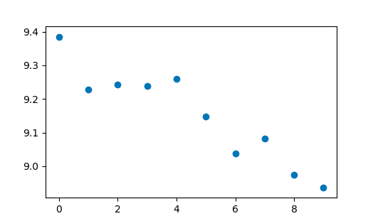 Linear sample
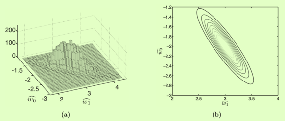 Likelihood function In the picture above, increasing causes a decrease in so we might expect the off-diagonal elements in the covariance matrix to be negative.
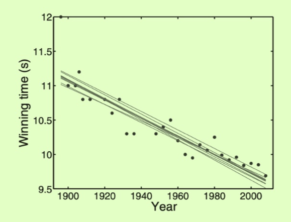 Diagonal Elements
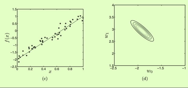 Off Diagonal Elements
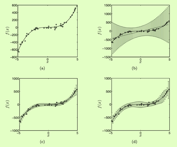 All models
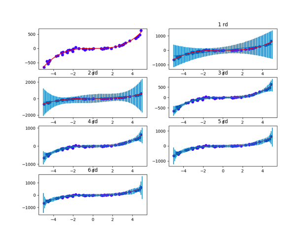 Simulation results