The Bayesian Approach To Machine Learning

---

The likelihood

$p ( \mathbf { t } | \mathbf { w } , \mathbf { X } , \sigma ^ { 2 } ) = \mathcal { N } \left( \mathbf { X } \mathbf { w } , \sigma ^ { 2 } \mathbf { I } _ { N } \right)$

The prior

$p ( \mathbf { w } | \boldsymbol { \mu } _ { 0 } , \mathbf { \Sigma } _ { 0 } ) = \mathcal { N } \left( \boldsymbol { \mu } _ { 0 } , \mathbf { \Sigma } _ { 0 } \right)$ We need to choose $\boldsymbol { \mu } _ { 0 }$ and $\boldsymbol { \Sigma } _ { 0 }$

The posterior

$\begin{aligned} p ( \mathbf { w } | \mathbf { t } , \mathbf { X } , \sigma ^ { 2 } ) & \propto p ( \mathbf { t } | \mathbf { w } , \mathbf { X } , \sigma ^ { 2 } ) p ( \mathbf { w } | \boldsymbol { \mu } _ { 0 } ) \\ = & \frac { 1 } { ( 2 \pi ) ^ { N / 2 } \left| \sigma ^ { 2 } \mathbf { I } \right| ^ { 1 / 2 } } \exp \left( - \frac { 1 } { 2 } ( \mathbf { t } - \mathbf { X } \mathbf { w } ) ^ { \top } \left( \sigma ^ { 2 } \mathbf { I } \right) ^ { - 1 } ( \mathbf { t } - \mathbf { X } \mathbf { w } ) \right) \\ & \times \frac { 1 } { ( 2 \pi ) ^ { N / 2 } \left| \mathbf { \Sigma } _ { 0 } \right| ^ { 1 / 2 } } \exp \left( - \frac { 1 } { 2 } \left( \mathbf { w } - \boldsymbol { \mu } _ { 0 } \right) ^ { \top } \mathbf { \Sigma } _ { 0 } ^ { - 1 } \left( \mathbf { w } - \boldsymbol { \mu } _ { 0 } \right) \right) \end{aligned}$

$\begin{aligned} \propto & \exp \left( - \frac { 1 } { 2 \sigma ^ { 2 } } ( \mathbf { t } - \mathbf { X } \mathbf { w } ) ^ { \top } ( \mathbf { t } - \mathbf { X } \mathbf { w } ) \right) \\ & \times \exp \left( - \frac { 1 } { 2 } \left( \mathbf { w } - \boldsymbol { \mu } _ { 0 } \right) ^ { \top } \mathbf { \Sigma } _ { 0 } ^ { - 1 } \left( \mathbf { w } - \boldsymbol { \mu } _ { 0 } \right) \right) \\ = & \exp \left\{ - \frac { 1 } { 2 } \left( \frac { 1 } { \sigma ^ { 2 } } ( \mathbf { t } - \mathbf { X } \mathbf { w } ) ^ { \top } ( \mathbf { t } - \mathbf { X } \mathbf { w } ) + \left( \mathbf { w } - \boldsymbol { \mu } _ { 0 } \right) ^ { \top } \mathbf { \Sigma } _ { 0 } ^ { - 1 } \left( \mathbf { w } - \boldsymbol { \mu } _ { 0 } \right) \right) \right\} \end{aligned}$

$p ( \mathbf { w } | \mathbf { t } , \mathbf { X } , \sigma ^ { 2 } ) \propto \exp \left\{ - \frac { 1 } { 2 } \left( - \frac { 2 } { \sigma ^ { 2 } } \mathbf { t } ^ { \top } \mathbf { X } \mathbf { w } + \frac { 1 } { \sigma ^ { 2 } } \mathbf { w } ^ { \top } \mathbf { X } ^ { \top } \mathbf { X } \mathbf { w } + \mathbf { w } ^ { \top } \mathbf { \Sigma } _ { 0 } ^ { - 1 } \mathbf { w } - 2 \boldsymbol { \mu } _ { 0 } ^ { \top } \mathbf { \Sigma } _ { 0 } ^ { - 1 } \mathbf { w } \right) \right\}$

$\begin{aligned} p ( \mathbf { w } | \mathbf { t } , \mathbf { X } , \sigma ^ { 2 } ) & = \mathcal { N } \left( \boldsymbol { \mu } _ { \mathbf { w } } , \mathbf { \Sigma } _ { \mathbf { w } } \right) \\ & \propto \exp \left( - \frac { 1 } { 2 } \left( \mathbf { w } - \boldsymbol { \mu } _ { \mathbf { w } } \right) ^ { \top } \mathbf { \Sigma } _ { \mathbf { w } } ^ { - 1 } \left( \mathbf { w } - \boldsymbol { \mu } _ { \mathbf { w } } \right) \right) \\ & \propto \exp \left\{ - \frac { 1 } { 2 } \left( \mathbf { w } ^ { \top } \mathbf { \Sigma } _ { \mathbf { w } } ^ { - 1 } \mathbf { w } - 2 \boldsymbol { \mu } _ { \mathbf { w } } ^ { \top } \mathbf { \Sigma } _ { \mathbf { w } } ^ { - 1 } \mathbf { w } \right) \right\} \end{aligned}$

The terms linear and quadratic in w in equations must be equal, so
$\Rightarrow$ $\begin{aligned} \mathbf { w } ^ { \top } \mathbf { \Sigma } _ { \mathbf { w } } ^ { - 1 } \mathbf { w } & = \frac { 1 } { \sigma ^ { 2 } } \mathbf { w } ^ { \top } \mathbf { X } ^ { \top } \mathbf { X } \mathbf { w } + \mathbf { w } ^ { \top } \mathbf { \Sigma } _ { 0 } ^ { - 1 } \mathbf { w } \\ & = \mathbf { w } ^ { \top } \left( \frac { 1 } { \sigma ^ { 2 } } \mathbf { X } ^ { \top } \mathbf { X } + \mathbf { \Sigma } _ { 0 } ^ { - 1 } \right) \mathbf { w } \end{aligned}$ $\boldsymbol { \Sigma } _ { \mathbf { w } } = \left( \frac { 1 } { \sigma ^ { 2 } } \mathbf { X } ^ { \top } \mathbf { X } + \mathbf { \Sigma } _ { 0 } ^ { - 1 } \right) ^ { - 1 }$

and $\begin{aligned} - 2 \boldsymbol { \mu } _ { \mathrm { w } } ^ { \top } \mathbf { \Sigma } _ { \mathrm { w } } ^ { - 1 } \mathbf { w } & = - \frac { 2 } { \sigma ^ { 2 } } \mathbf { t } ^ { \top } \mathbf { X } \mathbf { w } - 2 \boldsymbol { \mu } _ { 0 } ^ { \top } \boldsymbol { \Sigma } _ { 0 } ^ { - 1 } \mathbf { w } \\ \boldsymbol { \mu } _ { \mathbf { w } } ^ { \top } \mathbf { \Sigma } _ { \mathbf { w } } ^ { - 1 } \mathbf { w } & = \frac { 1 } { \sigma ^ { 2 } } \mathbf { t } ^ { \top } \mathbf { X } \mathbf { w } + \boldsymbol { \mu } _ { 0 } ^ { \top } \mathbf { \Sigma } _ { 0 } ^ { - 1 } \mathbf { w } \end{aligned}$ $\boldsymbol { \mu } _ { \mathbf { w } } ^ { \top } \boldsymbol { \Sigma } _ { \mathbf { w } } ^ { - 1 } = \frac { 1 } { \sigma ^ { 2 } } \mathbf { t } ^ { \top } \mathbf { X } + \boldsymbol { \mu } _ { 0 } ^ { \top } \boldsymbol { \Sigma } _ { 0 } ^ { - 1 }$ $\boldsymbol { \mu } _ { \mathrm { w } } ^ { \mathrm { T } } \boldsymbol { \Sigma } _ { \mathrm { w } } ^ { - 1 } \boldsymbol { \Sigma } _ { \mathrm { w } } = \left( \frac { 1 } { \sigma ^ { 2 } } \mathbf { t } ^ { \top } \mathbf { X } + \boldsymbol { \mu } _ { 0 } ^ { \top } \boldsymbol { \Sigma } _ { 0 } ^ { - 1 } \right) \boldsymbol { \Sigma } _ { \mathrm { w } }$ $\boldsymbol { \mu } _ { \mathbf { w } } ^ { \top } = \left( \frac { 1 } { \sigma ^ { 2 } } \mathbf { t } ^ { \top } \mathbf { X } + \boldsymbol { \mu } _ { 0 } ^ { \top } \mathbf { \Sigma } _ { 0 } ^ { - 1 } \right) \boldsymbol { \Sigma } _ { \mathbf { w } }$ $\mu _ { \mathrm { w } } = \Sigma _ { \mathrm { w } } \left( \frac { 1 } { \sigma ^ { 2 } } \mathbf { X } ^ { \mathrm { T } } \mathbf { t } + \mathbf { \Sigma } _ { 0 } ^ { - 1 } \boldsymbol { \mu } _ { 0 } \right)$

import numpy as np
import random
import pylab as plt

def gaussian2d(mu,sigma,xvals,yvals):
    const = (1.0/(2.0*np.pi))*(1.0/np.sqrt(np.linalg.det(sigma)))
    si = np.linalg.inv(sigma)
    xv = xvals-mu[0]
    yv = yvals-mu[1]
    return const * np.exp(-0.5*(xv*xv*si[0][0] + xv*yv*si[1][0] + yv*xv*si[0][1] + yv*yv*si[1][1]))

if __name__ == '__main__':
    data = np.loadtxt('olympic100m.txt',delimiter=',')
    x = data[:,0][:,None]
    t = data[:,1][:,None]
    x = x - x[0]
    x/= 4.0
    t = t # This is already a vector!
    inputx = x.reshape(len(x),1)
    X = np.array([[1,inputx[0]]])
    T = np.array([t[0]])
    sig = np.array([[100,0],[0,5]])
    myu = np.array([[0],[0]])
    xp = np.arange(-30,30,0.1)
    yp = np.arange(-10,10,0.1)
    Xp,Yp = np.meshgrid(xp,yp)
    Z = gaussian2d(myu,sig,Xp,Yp)
    #CS = plt.contour(Xp,Yp,Z,20,colors='k')
    #plt.xlabel('w_0')
    #plt.ylabel('w_1')
    sig_sq = 2
    plt.figure()
    plt.scatter(x,t)
    #Y = y.reshape(len(y),1)
    count = 0
    xpsub = np.arange(9,13,0.02)
    ypsub = np.arange(-0.5,0.5,0.02)
    Xpsub,Ypsub = np.meshgrid(xp,yp)
    for addx, addt in zip(inputx[1:], t[1:]):
        #print(X,T)
       count += 1
       T = np.vstack((T,addt))
       X = np.vstack((X,[1,addx]))
       #signew = np.linalg.inv((1.0/sig_sq)*np.dot(X.T,X) + np.linalg.inv(sig))
       #myunew = np.dot(signew,(1.0/sig_sq)*np.dot(X.T,T) + np.dot(np.linalg.inv(sig),myu))
       signew = np.linalg.inv((1.0/sig_sq)*X.T@X + np.linalg.inv(sig))
       myunew = signew@((1.0/sig_sq)*X.T@T + np.linalg.inv(sig)@myu)
       #print(myunew)
       if count%2== 0:
        plt.figure()
        plt.subplot(1,2,1)
        xl = np.linspace(-5,30,100)
        xline = xl.reshape(len(xl),1)
        xline = np.hstack((np.ones_like(xline),xline))
        yline = xline@myunew
        plt.plot(xl, yline)
        plt.scatter(x,t)

        plt.subplot(1,2,2)
        zposterior = gaussian2d(myunew, signew, Xpsub, Ypsub)
        cs = plt.contour(Xp, Yp,Z,20, colors = 'k')
        cs = plt.contour(Xpsub, Ypsub, zposterior,colors='r')
        plt.xlim([9,13])
        plt.ylim([-0.5,0.5])
        plt.title('First' + str(count) + ' points, contours')
    plt.show()

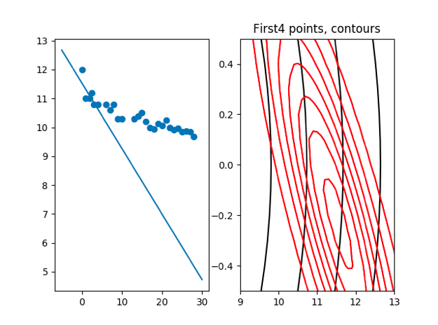
$cov: [ 1.47783251, -0.82101806 ]$ $[ - 0.82101806, 0.826491521 ]$ $\mu:$ $[ [ 11.57635468 ]$ $[ - 0.32019704 ] ]$

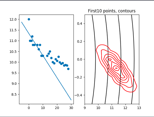
$cov: [ 0.6722373, - 0.12130803 ]$ $[ - 0.12130803, 0.03266264 ]$ $\mu:$ $[ [ 11.32030208 ]$ $[ - 0.09280969 ] ]$

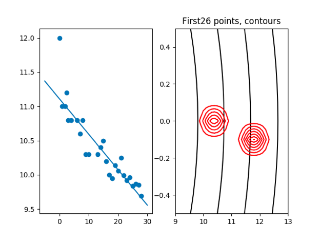
$cov:$ $[ 0.26539973 - 0.01359028 ]$ $[ - 0.01359028, 0.00096507 ]$

we can see that the cov is becomming more and more small with the incresing of points, that means we are less affected by the prior $\mu$ and cov.

    plt.scatter(x,t)
    xnew = np.linspace(-5,50,100)
    xnew = xnew.reshape(len(xnew),1)
    xerror = np.ones_like(xnew)
    #for m in range(1,i+1):
    xerror = np.hstack((xerror,xnew))
    inverse = np.linalg.inv(X.T@X)
    newsigma = sig_sq*xerror@inverse@xerror.T
    newsigma = np.diag(newsigma)
    plt.errorbar(xnew,xerror@myunew,yerr=newsigma)
    plt.show()

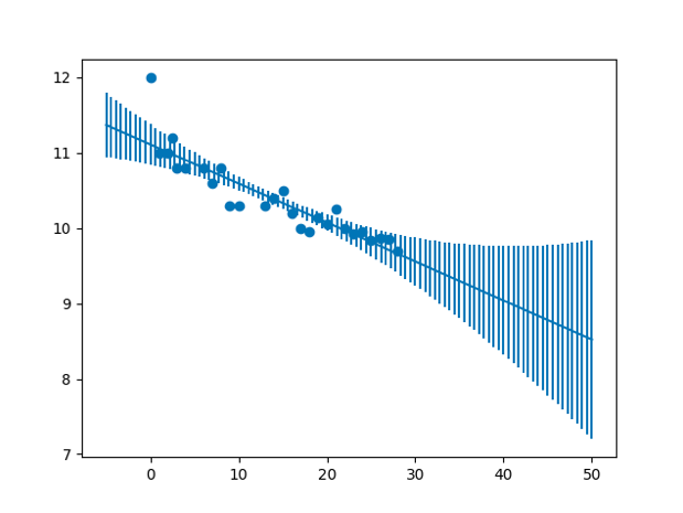Variance of the model

---

You May Also Enjoy

How To Train Multiple Model In One Time With Sklearn --Machine Learning

A Least Squares Approach --Machine Learning --Math

Linear Modeling - A Maximum Likelihood Approach --Machine Learning --Math

An Introduction To ESN --Math

Modeling With NMF And SVD --Machine Learning --Math

Feature Engineering For Machine Learning --Machine Learning

Welcome to share or comment on this post: