2019 August 07 Reinforcement Learning, Math

An Easy Way To Understand Temporal-Difference Learning In Reinforcement Learning

Introduction

Temporal-Difference (TD) learning is an very important part in reinforcement learning, which is practical in real world applications sinci it can learn from experience by interacting with environment, or directly learn from episodes generated by other policy, robot, or human. Comparing to Monte Carlo learning, which we’ve introduced in the last post: An Easy Way To Understand Monte Carlo Learning In Reinforcement Learning, TD has more advantages.

In this post, I’ll show you how to understand and use TD with minimal math and programming knowledge, in an easy way.

What is TD learning - Intuition?

Imagine, our old friend yyxsb is playing LOL, but he is too stupid to win. Thus we decide to develop a robot to help him. Instead, yyxsb will collect data for us to analyze. Here he has two options:

Play the game and record all the data like [state (money, position, etc.), action(how to move), reward (loss: 0, win: 1)] for every timestamp. The collected episodes are provided.
Play the game, and our robot learn from it at the same time.

If we want to use Monte Carlo learning, we have to choose option $1$ because if the game doesn’t terminate, the policy cannot be updated ( $G(s)$ cannot be calculated if complete episode is not been provided). While for TD learning, we can update the parameters when yyxsb is playing (option $2$ ), which means: every timestamp we collect the data, and use the data to update our robot parameters, look great, right? Well, that’s all of TD learning. Of course, TD can also choose option $1$ , and I will show you how to complete it in python code. Why I choose option $1$ in this post for TD learning? Because in other posts on the net, they all choose option $2$ , I want to show you some different.

Why do we need to introduce TD learning?

Readers of this post must know about dynamic programming (DP) and Monte Carlo (MC) learning. Here we talk about the advantages and disadvantages of DP and MC learning.

DP can update estimates based in part on other learned estimates, without waiting for a final outcome, which means they bootstrap. Like this formula, to calculate $v_{k+1}(s)=\sum_{a \in \mathcal{A}} \pi(a | s)\left(\mathcal{R}_{s}^{a}+\gamma \sum_{s^{\prime} \in \mathcal{S}} \mathcal{P}_{s s^{\prime}}^{a} v_{k}\left(s^{\prime}\right)\right)$ , we need to calculate the $v_{k}(s^{\prime})$ first, which means: if we want to understand now, we need to understand the near future! That’s bootstrap! However, DP assumes the whole environment model is provided, which is almost impossible in practice. Bootstrapping
MC can learn directly from episodes of experience, and it model-free, which means it doesn’t need knowledge of MDP. However, MC learns from complete episodes, which means it can only apply to episodic MDPs, also have to wait a episode ends, then MC can start learning.

Bootstrap method can calculate state now from the next state, but model free is also very attractive in practice, then the text question is: Is there a method that bootstrap and model free? Then anwser is yes, that’s TD. I mean TD can calculate state from the estimated next state, also it’s model free and can learn from episode. Since it’s a bootstrapping method, TD can learn from infinite episode or continuing (non-terminating) environments, which is actually online learning.

How to understand TD learning?

Do you remember the Monte Carlo learning, whose simple formula is: $V\left(S_{t}\right) \leftarrow V\left(S_{t}\right)+\alpha\left[G_{t}-V\left(S_{t}\right)\right]$ where $G_{t}$ is the actual return following time $t$ , and $\alpha$ is a constant step-size parameter (we can determin it ourselves). Monte Carlo uses an estimate of the actual return (average many samples). Only if the episode is terminate we can calculate $G_{t}$ , thus MC methods are often very slow. What? you cannot understand why? Then you should read this post first

So whats’ the TD leaning? Well, in a simple way, $V\left(S_{t}\right) \leftarrow V\left(S_{t}\right)+\alpha\left[R_{t+1}+\gamma V\left(S_{t+1}\right)-V\left(S_{t}\right)\right] \tag{1}$ Here is some pseudocode:

pi = init_pi()
V = init_V()
for i in range(NUM_ITER):
    s = init_state()
    episode = init_episode(s)
    while episode:
        prev_s = s
        action = get_action(pi, V)
        reward, s = episode.run(action)
        V(prev_s) += alpha * (reward + gamma * V(s) - V(prev_s))

You see what? The $G_{t}$ we used in $(1)$ is replaced by $R_{t+1} + \gamma V(S_{t+1})$ . Why could we do that?

$\begin{aligned} V^{\pi}(s) &=E_{\pi}\left\{R_{t} | s_{t}=s\right\} \tag{2} \\ &=E_{\pi}\left\{\sum_{k=0}^{\infty} \gamma^{k} r_{t+k+1} | s_{t}=s\right\} \\ &=E_{\pi}\left\{r_{t+1}+\gamma \sum_{k=0}^{\infty} \gamma^{k} r_{t+k+2} | s_{t}=s\right\} \\ &=E_{\pi}\left\{r_{t+1}+\gamma V^{\pi}\left(s_{t+1}\right) | s_{t}=s\right\} \\ &=\sum_{a} \pi(s, a) \sum_{s^{\prime}} P_{s s^{\prime}}^{a}\left[R_{s s^{\prime}}^{a}+\gamma V^{\pi}\left(s^{\prime}\right)\right] \end{aligned}$ $(2)$ is the proof, in fact, we just use an estimate of reward to estimate tha state value now, again, it bootrstraps! Notice that the first line of $(2)$ is MC learning, the second from the lats line is used in TD learning, and the last line is DP. From $(2)$ we could see that MC method is an unbiased estimate of $v_{\pi}(S_{t})$ , and TD method is biased since we use $R_{t+1} + \gamma V_{S_{t+1}}$ instead of $R_{t+1} + \gamma v_{\pi}(S_t+1)$ . Why? Because we don’t know the real $v_{\pi}(S_{t+1})$ , but we can estimate $V(S_{t+1})$ from episodes. Also TD method has much lower variance than MC method since $R_{t+1} + \gamma V(S_{t+1})$ only depends on one random action, transition, reward, while $G_{t}=R_{t+1}+\gamma R_{t+2}+\ldots+\gamma^{T-1} R_{T}$ depends on many.

If we choose $G_{t} = R_{t+1} + \gamma V(S_{t+1})$ in TD learning, we call them $\mathit{TD}(0)$ ; if we choose $G_{t} = R_{t+1} + \gamma R_{t+2} + \gamma^{2}V(S_{t+2})$ , we call them $\mathit{TD}(1)$ . Of course $\mathit{TD}(\infty)$ is MC learning, since in this time $G_{t} = R_{t+1}+\gamma R_{t+2}+\ldots+\gamma^{T-1} R_{T}$ . In this post, I will only show you $\mathit{TD}(0)$ , because understand it only is enough.

We note that in $(1)$ , $\mathit{TD}(0)$ is actually update a sort of error, measuring the di↵erence between the estimated value of $S_{t}$ and the better estimate $R_{t+1} + V(S_{t+1})$ . We call this quantity $\mathit{TD}$ error. And definite it as $\delta_{t} \doteq R_{t+1}+\gamma V\left(S_{t+1}\right)-V\left(S_{t}\right)$ .

How to estimate state values / state action values?

It’s very easy, just iterate to update $V(S)$ . Here is the algorithm. 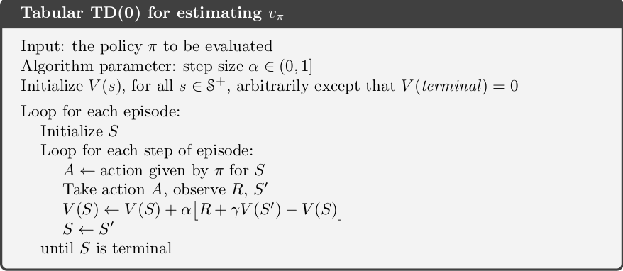Calculate $V(S)$ given $\pi$

How to get optimal policy?

In TD learning, we also have two ways:

On-policy learning: Sarsa
Off-policy learning: Q-learning

How to use Sarsa?

It’s very intuitive: we just update the $Q$ like what we have done in MC learning. Here we need to use $S_{t}, A_{t}, R_{t+1}, S_{t+1}, A_{t+1}$ , that’s Sarsa for the algorithm. 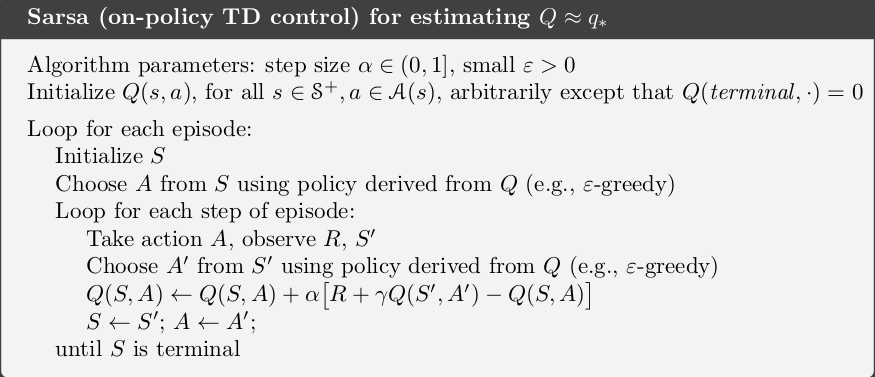Sarsa algorithm

Since it’s relatively easy, we don’t show python code here.

How to use Q-learning?

Here is the main hero today: Q-learning. $Q\left(S_{t}, A_{t}\right) \leftarrow Q\left(S_{t}, A_{t}\right)+\alpha\left[R_{t+1}+\gamma \max _{a} Q\left(S_{t+1}, a\right)-Q\left(S_{t}, A_{t}\right)\right] \tag{3}$ $(3)$ will directly approximates $q_{*}$ , the optimal action-value fuction, independent of the policy being followed. However, all that is required for correct convergence is that all pairs continue to be updated.

And here is the algorithm, easy and beautiful. 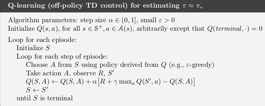Q_learning algorithm

A simple eaxmple to show you how to Q-learning

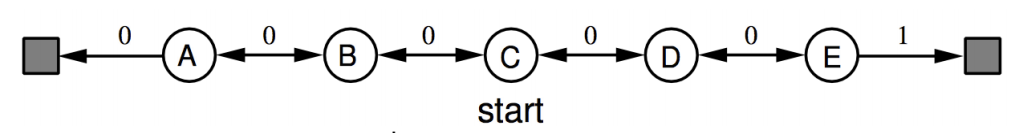Random Walk Example

Robot start from C, and can randomly choose go left or right. the grey square means terminate. From E to $T$ (terminate), the robot can get reward $1$ , others are $0$ .

First we need to get some episode from a policy, here we use $\pi(\mathit{left}) = \pi(\mathit{right}) = 0.5$ to collect episodes. Here is the code:

S_A_trans = {'T': ['T','T'],
             'A': ['T','B'],
             'B': ['A','C'],
             'C': ['B','D'],
             'D': ['C','E'],
             'E': ['D','T']}
Reward_table = {"TT":0,"AT":0,"AB":0,"BA":0,"BC":0,"CB":0,"CD":0,"DC":0,"DE":0,"ED":0,"ET":1}
p_pi = 0.5  # possibility of choosing left is 0.5
l = 0 # for choose S_A_trans
r = 1
Action_table = {'l':0, 'r':1}
Action_table_reverse = {0:'l', 1:'r'}
def sample_episodes(numbers_needed):
    episodes = []
    for _ in range(numbers_needed):
        state_now = 'C'
        episode = []
        while state_now != 'T':
            if np.random.rand() < p_pi:
                action = 'l'
            else:
                action = 'r'
            state_next = S_A_trans[state_now][Action_table[action]]
            reward = Reward_table[state_now + state_next]
            episode.append(state_now)
            episode.append(action)
            episode.append(reward)
            
            state_now = state_next
        episode.append(state_now)  # add 'T'
        episodes.append(episode)
    return episodes
episodes = sample_episodes(1000)

For example, if we run sample_episodes(2), we can get [['C', 'l', 0, 'B', 'l', 0, 'A', 'l', 0, 'T'], ['C', 'l', 0, 'B', 'r', 0, 'C', 'r', 0, 'D', 'r', 0, 'E', 'l', 0, 'D', 'r', 0, 'E', 'l', 0, 'D', 'r', 0, 'E', 'r', 1, 'T']]

Then initilize the $Q$ :

Q = {"Tl":0, 'Tr':0, "Al":0, "Ar":0, "Bl":0, "Br":0, "Cl":0,"Cr":0, "Dl":0, "Dr":0, "El":0,"Er":1}
for state_action in Q:
    Q[state_action] = np.random.rand()
Q["Tl"] = 0
Q["Tr"] = 0

Then we can prefer Q-learning:

# Q learning
alpha = 0.1
gamma = 0.7
for episode in episodes:
    state_now = episode[0]
    for pos in range(0, len(episode), 3):
        action = episode[pos + 1 ]
        reward = episode[pos + 2]
        state_next = episode[pos + 3 ]    
        
        # Update Q
        Q[ state_now + action ] = Q[ state_now + action ] + alpha *( reward + gamma * max_Q_value(state_next, Q) - Q[ state_now + action ] )
        state_now = state_next
        if state_now == 'T':
            break
print(Q)

Result:
{'Tl': 0, 'Tr': 0, 'Al': 3.641070925429505e-24, 'Ar': 0.2400999999999992, 'Bl': 0.16806999999999933, 'Br': 0.3429999999999991, 'Cl': 0.2400999999999992, 'Cr': 0.4899999999999991, 'Dl': 0.3429999999999991, 'Dr': 0.6999999999999991, 'El': 0.4899999999999991, 'Er': 0.9999999999999996}

It’s obvious that we should choose r action for any state with a greedy policy.

Here is the full script.

import numpy as np
S_A_trans = {'T': ['T','T'],
             'A': ['T','B'],
             'B': ['A','C'],
             'C': ['B','D'],
             'D': ['C','E'],
             'E': ['D','T']}
Reward_table = {"TT":0,"AT":0,"AB":0,"BA":0,"BC":0,"CB":0,"CD":0,"DC":0,"DE":0,"ED":0,"ET":1}
p_pi = 0.5  # possibility of choosing left is 0.5
l = 0 # for choose S_A_trans
r = 1
Action_table = {'l':0, 'r':1}
Action_table_reverse = {0:'l', 1:'r'}
def sample_episodes(numbers_needed):
    episodes = []
    for _ in range(numbers_needed):
        state_now = 'C'
        episode = []
        while state_now != 'T':
            if np.random.rand() < p_pi:
                action = 'l'
            else:
                action = 'r'
            state_next = S_A_trans[state_now][Action_table[action]]
            reward = Reward_table[state_now + state_next]
            episode.append(state_now)
            episode.append(action)
            episode.append(reward)
            
            state_now = state_next
        episode.append(state_now)  # add 'T'
        episodes.append(episode)
    return episodes

def max_Q_value(state_next, Q):
    action_best = 'l' if Q[ state_next + 'l' ] > Q[ state_next + 'r' ] else 'r'
    return Q[ state_next + action_best ]

Q = {"Tl":0, 'Tr':0, "Al":0, "Ar":0, "Bl":0, "Br":0, "Cl":0,"Cr":0, "Dl":0, "Dr":0, "El":0,"Er":1}
for state_action in Q:
    Q[state_action] = np.random.rand()
Q["Tl"] = 0
Q["Tr"] = 0


episodes = sample_episodes(1000)

# Q learning
alpha = 0.1
gamma = 0.7
for episode in episodes:
    state_now = episode[0]
    for pos in range(0, len(episode), 3):
        action = episode[pos + 1 ]
        reward = episode[pos + 2]
        state_next = episode[pos + 3 ]    
        
        # Update Q
        Q[ state_now + action ] = Q[ state_now + action ] + alpha *( reward + gamma * max_Q_value(state_next, Q) - Q[ state_now + action ] )
        state_now = state_next
        if state_now == 'T':
            break
print(Q)

Summary

In this post we introduced a new kind of learning method, temporal-difference (TD) learning, and showed how it can be applied to the reinforcement learning problem. In the future post, we will talk about how to combine deep learning with Q-learning: DQN. Please check this post: How To Play Cart Pole Game with Temporal Difference Learning By Pytorch?

An Easy Way To Understand Temporal-Difference Learning In Reinforcement Learning

Introduction

What is TD learning - Intuition?

Why do we need to introduce TD learning?

How to understand TD learning?

How to estimate state values / state action values?

How to get optimal policy?

How to use Sarsa?

How to use Q-learning?

A simple eaxmple to show you how to Q-learning

Summary

References

You May Also Enjoy

A Least Squares Approach --Math

Linear Modeling - A Maximum Likelihood Approach --Math

The Bayesian Approach To Machine Learning --Math

An Introduction To ESN --Math

Modeling With NMF And SVD --Math

Bounding Box Regression --Math