An Introduction To ESN

---

ESN

Intuitive

1. An instance of the more general concept of reservoir computing.
2. No problems of training a traditional RNN.
3. A large reservoir of sparsely connected neurons using a sigmoidal transfer function(relative to input size, like 1000 units).
4. Connections in the reservoir are assigned once and are completely random.
5. The reservoir weights do not get trained.
6. Input neurons are connected to the reservoir and feed the input activations into the reservoir - these too are assigned untrained random weights.
7. The only weights that are trained are the output weights which connect the reservoir to the output neurons.
8. Sparse random connections in the reservoir allow previous states to “echo” even after they have passed.
9. Input/output units connect to all reservoir units.
10. The output layer learns which output has to belong to a given reservoir state. - Training becomes a linear regression task.

Model

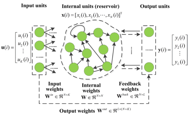
General model

$\begin{aligned} \mathbf{r}(t+1) &=f\left(W_{\text { res }}^{\text { res }} \mathbf{r}(t)+W_{\text { inp }}^{\text { res }} \mathbf{u}(t)+W_{\text { out }}^{\text { res }} \mathbf{y}(t)+W_{\text { bias }}^{\text { res }}\right) \\ \widehat{\mathbf{y}}(t+1) &=W_{\text { res }}^{\text { out }} \mathbf{r}(t+1)+W_{\text { inp }}^{\text { out }} \mathbf{u}(t)+W_{\text { out }}^{\text { out }} \mathbf{y}(t)+W_{\text { bias }}^{\text { out }} \end{aligned}$ If we choose $f = tanh$, we can write it like: $\begin{aligned} \mathbf{r}(t+\Delta t)=(1-\alpha) \mathbf{r}(t)+\alpha \tanh \left(\mathbf{A} \mathbf{r}(t)+\mathbf{W}_{i n} \mathbf{u}(t)+\xi 1\right) \end{aligned}$ Here:

• $u(t)$: input of time t.
• $\begin{aligned}W_{i np}\end{aligned}$: weights of input layer.
• $K$: num(input layer nodes)
• $\begin{aligned}\alpha\end{aligned}$: leakage rate, control the update speed of reservoir nods.
• $r$: reservoir state vector, recoding weight information of each reservoir node.
• $A$: weighted adjacency matrix, usually a sparse matrix, use $\text { Erdós-Rényi }$ to generate.
• $\begin{aligned} \mathbf{W}_{i n}\end{aligned}$: (N,M) matrix, to change M-dim signals into reservoir computable format.
• $\begin{aligned} \mathbf{u}(t)\end{aligned}$: input signal, M-dim.
• $\begin{aligned}\xi\end{aligned}$: bias.

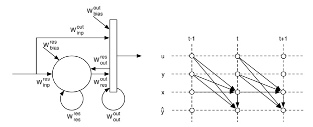
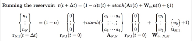Running the reservoir

Here, all weights matrices to the reservoir ($W^{\text { res }}$) are initialized at random, while all connections to the output ($W^{\text { out }}$) are trained.

Train

1. Initial period

Update reservoir states $R$

for t in range(trainLen):
  u = input_signal[t]
  r = (1 − alpha) ∗ r + alpha ∗ np.tanh(np.dot(A, r) + np.dot(Win, u) + bias)
  if t >= initLen:
    R[:, [t − initLen]] = np.vstack((u, r))[:, 0]

2. Training peroid

After collecting all these states, use ridge regression to train parameters. $\begin{aligned} W_{o u t}^{*}=\mathbf{S R}^{T}\left(\mathbf{R} \mathbf{R}^{T}+\beta \mathbf{I}\right)^{-1} \end{aligned}$ $S$ means target matrix

Test

To test reservoir: $\begin{aligned} \hat{\mathbf{s}}=\mathbf{W}_{o u t} \mathbf{r}(t) \end{aligned}$

S = np.zeros((P, testLen))
u = input_signal[trainLen]
for t in range(testLen):
  r = (1 − alpha) ∗ r + alpha ∗ np.tanh(np.dot(A, r) + np.dot(Win, u) + bias) 
  s = np.dot(Wout, np.vstack((u, r)))
  S[:, t] = s
  u=s

Evaluation

RMS(root mean square) error.

Others

Echo state property

Input now has bigger effect on inner states than previous input or states.
That means it has to dismiss initial states when stable.
To meet ESP, the biggest eigenvalue of $W^{\text { res }}$ has to closer to 1 and less than 1.
(in program, make the max eigenvalue scales to 0.99 is ok)

Reference

1. An overview of reservoir computing: theory, applications and implementations
2. Introduction to reservoir computing
3. ゼロから作るReservoir Computing
4. Echo state network

---

You May Also Enjoy

A Least Squares Approach --Math

Linear Modeling - A Maximum Likelihood Approach --Math

The Bayesian Approach To Machine Learning --Math

Modeling With NMF And SVD --Math

Bounding Box Regression --Math

An Easy Way To Understand Temporal-Difference Learning In Reinforcement Learning --Math

Welcome to share or comment on this post: