How To Play Cart Pole Game with Temporal Difference Learning By Pytorch?

---

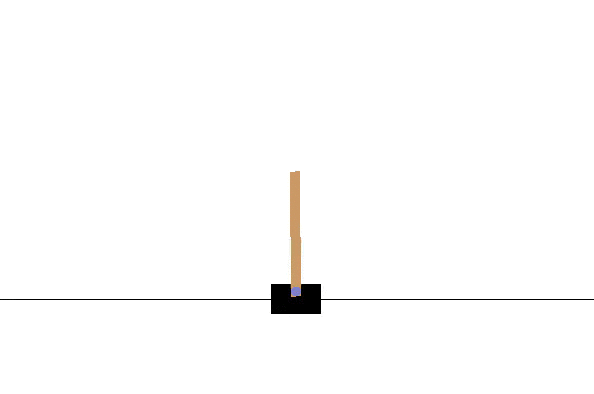Cart Pole game played by reinforcement learning algorithm (DQN)

Introduction

We’ve learned how Temporal-Difference learning works in the last post, if you don’t, please check this post: Easy TD introduction. However, since in practice the numbers of states maybe infinite, which means the table method we’ve used untill now doesn’t work (we just use a table to store all states and actions).

In this post I’ll show you how to solve the problem above, and use Q-learning to play cart pole game by pytorch in an very easy and clear way. The gif above is the final result, if you want to know why and how it works, don’t miss this post.

Why we don’t use tables to store states any more?

Q-learning is about creating the cheat sheet Q.

Usually, we can store the $Q(S,A)$ table in this format.

States	Action $a_{1}$	Action $a_{2}$	…
$S_{1}$	$Q(S_{1},a_{1})$	$Q(S_{1},a_{2})$	$Q(S_{...},a_{...})$
$S_{2}$	$Q(S_{2},a_{1})$	$Q(S_{2},a_{2})$	$Q(S_{...},a_{...})$
$S_{...}$	$Q(S_{...},a_{1})$	$Q(S_{...},a_{2})$	$Q(S_{...},a_{...})$

However, as you can see, when the states grows, the computer may have no enough space, or cannot search a table timely. I mean, for example, if the state is over $10^{80}$, it’s impossible to store or iterate that table.

Thus we need to approximate the $V_{\pi}(s)$ or $Q_{\pi}(s)$ function, and we hope the approximation function can be generalized well for $V_{\pi}(s)$ or $Q_{\pi}(s)$. We have many ways to do so, in this post, I will only show you how to use neural network to approximate $Q_{\pi}(s)$ for $s \in \mathcal{S}$ . What? You mean why? Well, if we have a neural network that can tell us the $Q$ value for all state-action pairs, then we can use greedy policy to choose the best actions. If we just updathe the neural network untill it can approximate $Q_{*}$ (optimal $Q$), then the biggest output of $Q_{*}$ is optimal action. That’s our target!

Value function approximation

Since DQN is still value function based method, we need to compute value function to get the policy, and use the concept of GPI to get optimal policy.

How to use neural networks to represent $Q^{*}$

In general, we have two methods:

1. $(s,a)$ as input, output is $Q(s,a)$, one output
2. $s$ as input, output as $Q(s,a_{n})$, which has $n$ outputs corresponding to each action

Method $1$ is often used in continous actions, and method $2$ is often used for discrete actions. In this post, I will use method $2$. Then we can use $f_{Q_{*}}(s, a; \theta)$ to represent $Q_{*}(s,a)$ with method $2$.

How to update value function?

The next question is how to update the neural networks. We’ll use gradient descent to update our network.

Then we need to make a loss function! We write it as $C(\theta)$. The goal of our neural network is to approximate $Q_{*}$, right? Recall that the $\mathit(TD)$ error $\left[R_{t+1}+\gamma \max _{a} Q\left(S_{t+1}, a\right)-Q\left(S_{t}, A_{t}\right)\right]$, when $\mathit{TD}$ error converges to $0$, that meas $Q$ is optimal. That is: we use episode to estimate a reward to subtract the $Q$ we have now, and use the error to update that $Q$, finally we can get $Q_{*}$. How amazing!

Also, in neural network, we can use designate $C (\theta) = |R\left(s, a, s^{\prime}\right)+\gamma \max _{a^{\prime}} f_{Q_{*}}\left(s^{\prime}, a^{\prime} ; \theta\right)-f_{Q_{*}}(s, a ; \theta)|$, which is a $\mathit{l1}$ loss. In practice, we often choose MSE error.

$\theta \leftarrow \theta-\eta \nabla_{\theta} C \tag{1}$ And $C(\theta)=[R(s, a, s^{\prime})+\gamma \max _{a^{\prime}} f_{Q_{*}}(s^{\prime}, a^{\prime} ; \theta)-f_{Q_{*}}(s, a ; \theta)]^{2}$

Don’t worry about the gredients, deep learning library will help use calculate them automatically.

Everything seems works fine, right?

Is the formula works in practice?

Well, unfortunately, if we use the formula above to update the neural network, it often diverges due to:

• Samples are correlated
  • In AI, we assume the data is independent and identically distributed randomly, we call it $\mathit{i.i.d}$. If, the data doesn’t meet $\mathit{i.i.d}$, then it may not converge. In reinforcement learning, since the episode is inherently correlated, like action $a$ will affect state $s_{1}$, and then make decision $b$.
• Non-stationary target
  • This means when the network is updated for current $a$, $f_{Q_{*}}(s^{\prime}, a^{\prime})$ will also change. For example, if our target is $1$, while every time we update the network, the target changes, then network cannot learn well. In this work, update $f_{Q_{*}}(s,a;\theta)$ will affect $R(s,a,s^{\prime}) + \gamma \max _{a^{\prime}} f_{Q_{*}}(s^{\prime},a^{\prime};\theta)$

In reinforcement learning, both the input and the target change constantly during the process and make training unstable.

Due to the two big problems, Q-learning usually cannot converge. DeepMind pubulished a paper in nature and tell us that we have methods to solve the problems above.

How to solve the problems above?

Experience Replay

This method is to solve the $\mathit{i.i.d}$ problem. That is: we just use a replay memory $\mathcal{D}$ to store recently seen transitions $(s,a,r,s^{\prime})$. In $\mathcal{D}$, we have many transitions, and every time we want to update the parameters, we can sample a mini-batch from $\mathcal{D}$ to update $\theta$.

With experinece replay, the network can often converge now. But very slow, since we still have a big problem need to solve.

Delayed Target Network

Since the question is how to avoid changing $\delta = R(s,a,s^{\prime}) + \gamma \max _{a^{\prime}} f_{Q_{*}}(s^{\prime},a^{\prime};\theta)$ when updating $f_{Q_{*}}(s,a;\theta)$, we can just use two neural network $\theta^{-}$ and $\theta$, one for $\delta (\theta^{-}) = R(s,a,s^{\prime}) + \gamma \max _{a^{\prime}} f_{Q_{*}}(s^{\prime},a^{\prime};\theta^{-})$ and another for $f_{Q_{*}}(s,a;\theta)$

Since $\theta^{-}$ and $\theta$ need to be the same network, we need to make $\theta^{-} \leftarrow \theta$ every $K$ like $100$ iterations.

Here is the algorithm from nature paper. Deep Q-learning with experience replay

Show me the code

In this section, I will show you how to use the algorithm above to play cart pole game with pytorch. Since I’ve tried to write the code corresponding to the algorithm in the paper, I recommend you read to code while seeing the algorithm. I think you will have a better understanding if you do so.

DQN

This is the $\theta$ we’ve just described. Here are some questions need to answer.

• Why don’t I choose ‘stronger’ network?
  • If the model has big capacity, then the network will over-fit after about 100 episodes.
• Why don’t I choose convolutional neural network?
  • Since this is to show you an easy way to play cart pole game with reinforcement learning algorithm, I don’t want to show too much knowledge here. Also, the gym module gives us the state in numeral format, it’s more convenient to use numeral format, isn’t it?

class DQN(torch.nn.Module):
    def __init__(self, observation_space, action_space):
        super(DQN, self).__init__()
        self.net = nn.Sequential(
            nn.Linear(observation_space, 20),
            nn.ReLU(inplace = True),
            nn.Linear(20, 20),
            nn.ReLU(inplace = True),
            nn.Linear(20, 10),
            nn.ReLU(inplace = True),
            nn.Linear(10, action_space),
        )

    def forward(self, observation):
        return self.net(observation)

Predict an action according to $\epsilon$-$\mathit{greedy}$ policy

Here the exploration_rate is decayed with time. That means, first exploring a lot, then less.

# @state is tensor
def predict(self, state):
    if np.random.rand() < self.exploration_rate:
        return random.randrange(self.action_space)

    q_values = self.Q_policy(state)[0]

    # best action
    max_q_index =  torch.max(q_values, 0).indices.numpy()
   # print(torch.max(q_values).detach().numpy())
    return max_q_index

Experience Replay

def experince_replay(self):
    if len(self.memory) < BATCH_SIZE:
        return
    batch = random.sample(self.memory, BATCH_SIZE)
    for state, action, reward, state_next, terminal in batch:
        self.optimizer.zero_grad()

        y = reward
        if not terminal:
            y = reward + GAMMA * torch.max( self.Q_target(state_next) )
        state_values = self.Q_policy(state)
        if action == 0:
            real_state_action_values = torch.sum(state_values * torch.FloatTensor([1.0, 0]))
        else:
            real_state_action_values = torch.sum(state_values * torch.FloatTensor([0, 1.0]))
        loss = self.lossFuc(y, real_state_action_values)

        loss.backward()
        self.optimizer.step()
    self.exploration_rate *= EXPLORATION_DECAY
    self.exploration_rate  = max(EXPLORATION_MIN, self.exploration_rate)

Here is the full script.

import gym
import numpy as np
import random
from collections import deque
import time

import torch
import torch.nn as nn
import torch.optim as optim
import torch.nn.functional as F
import copy

ENV_NAME = "CartPole-v1"

GAMMA = 0.95
LEARNING_RATE = 3e-4

MEMORY_SIZE = 1000000
BATCH_SIZE = 20

EXPLORATION_MAX = 1.0
EXPLORATION_MIN = 0.01
EXPLORATION_DECAY = 0.995

class DQN(torch.nn.Module):
    def __init__(self, observation_space, action_space):
        super(DQN, self).__init__()
        self.net = nn.Sequential(
            nn.Linear(observation_space, 20),
            nn.ReLU(inplace = True),
            nn.Linear(20, 20),
            nn.ReLU(inplace = True),
            nn.Linear(20, 10),
            nn.ReLU(inplace = True),
            nn.Linear(10, action_space),
        )

    def forward(self, observation):
        return self.net(observation)


class GameSolver:
    def __init__(self, observation_space, action_space):
        self.exploration_rate = EXPLORATION_MAX

        self.action_space = action_space
        self.memory = deque(maxlen=MEMORY_SIZE)
        self.Q_policy = DQN(observation_space, action_space)
        self.Q_target = copy.deepcopy(self.Q_policy)
        self.optimizer = optim.Adam(self.Q_policy.parameters(), lr = LEARNING_RATE)
        self.lossFuc = torch.nn.MSELoss()

    def remember(self, state, action, reward, next_state, done):
        self.memory.append((state, action, reward, next_state, done))

    def predict(self, state):
        if np.random.rand() < self.exploration_rate:
            return random.randrange(self.action_space)

        q_values = self.Q_policy(state)[0]

        # best action
        max_q_index =  torch.max(q_values, 0).indices.numpy()
       # print(torch.max(q_values).detach().numpy())
        return max_q_index

    def experince_replay(self):
        if len(self.memory) < BATCH_SIZE:
            return
        batch = random.sample(self.memory, BATCH_SIZE)
        for state, action, reward, state_next, terminal in batch:
            self.optimizer.zero_grad()

            y = reward
            if not terminal:
                y = reward + GAMMA * torch.max( self.Q_target(state_next) )
            state_values = self.Q_policy(state)
            if action == 0:
                real_state_action_values = torch.sum(state_values * torch.FloatTensor([1.0, 0]))
            else:
                real_state_action_values = torch.sum(state_values * torch.FloatTensor([0, 1.0]))
            loss = self.lossFuc(y, real_state_action_values)

            loss.backward()
            self.optimizer.step()
        self.exploration_rate *= EXPLORATION_DECAY
        self.exploration_rate  = max(EXPLORATION_MIN, self.exploration_rate)

def cartpole():
    env = gym.make(ENV_NAME)
    observation_space = env.observation_space.shape[0]
    action_space = env.action_space.n
    gameSolver = GameSolver(observation_space, action_space)
    run = 0
    while True:
        run += 1
        state = env.reset()
        state = torch.FloatTensor(np.reshape(state, [1, observation_space]))
        step = 0
        while True:
            step += 1
            env.render()
          #  time.sleep(0.05)
            action = gameSolver.predict(state)
            state_next, reward, terminal, info = env.step(action)
            reward = reward if not terminal else -reward * 10
            if step == 500:
                reward = 1000
            reward = torch.tensor(reward)
            state_next = torch.FloatTensor(np.reshape(state_next, [1, observation_space]))
            gameSolver.remember(state, action, reward, state_next, terminal)

            state = state_next

            if terminal:
                print ("Run: " + str(run) + ", exploration: " + str(gameSolver.exploration_rate) + ", score: " + str(step) )
                break
            gameSolver.experince_replay()
            if run % 3 == 0 or step % 100 == 0:
                gameSolver.Q_target = copy.deepcopy(gameSolver.Q_policy)

if __name__ == "__main__":
    cartpole()

Here is the result: 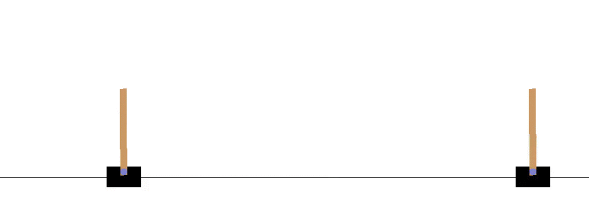Left: trained 50 episodes | Right: trained 100 episodes

Summary

In this post we introduced how to use neural networks to play Cart Pole game from math to algorithm, then to code! I think it’s amazing that math can be so useful, right? In the next post, I’ll show you how to play flappy bird with reinforcement learning that uses convolutional neural network to approximate $Q$ in It’s Really Easy To Play Flappy Bird Via Reinforcement Learning.

References

• Human-level control through deep reinforcement learning
• REINFORCEMENT LEARNING (DQN) TUTORIAL
• Deep Q-Network (DQN) video
• RL — DQN Deep Q-network
• SARSA Reinforcement Learning

---

You May Also Enjoy

It's Really Easy To Play Flappy Bird Via Reinforcement Learning --Reinforcement Learning --Application

An Easy Way To Understand Temporal-Difference Learning In Reinforcement Learning --Reinforcement Learning

Importance Sampling In Reinforcement learning --Reinforcement Learning

An Easy Way To Understand Monte Carlo Learning In Reinforcement Learning --Reinforcement Learning

An Easy Way To Understand Dynamic Programming In Reinforcement Learning --Reinforcement Learning

An Easy Way To Understand Markov Decision Process In Reinforcement Learning --Reinforcement Learning

Welcome to share or comment on this post: