An Easy Way To Understand Dynamic Programming In Reinforcement Learning

---

Introduction

Sometimes we have to learn something that we will never use in practice, like now.

Probably you will never use dynamic programming (DP) in your life, but understand it is necessary it provide a general idea to solve reinforcement learning problems. In this post, I will show you why and how dynamic programming works with little math and programming knowlege. Before read this post, ensure that you understand what is markov decision process, else please check this post: An Easy Way To Understad Markov Decision Process In Reinforcement Learning Since we will only learn the basic idea from this DP, thus I won’t introduce the whole things clearly here.

Why DP is introduced?

In the MDP post, we’ve talked about how to calculate the value function using a fixed policy, and given math equations that show the relationship between $v_{*}(s)$ and $q_{*}(s)$.

But, what can they do for us? In real applications, we only know state values that are not optimal, let alone the best policy. Thus, we need a way to get optimal state values or best policy. Dynamic Programming is a general solution.

How DP works?

Assumption for DP

• Optimal substructure
  • Optimal solution can be decomposed into subproblems
• Overlapping subproblems
  • Subproblems recur many times
  • Solutions can be cached and reused

In fact, markov decision processes satisfy both properties

• Bellman equation gives recursive decomposition
• Value function stores and reuses solutions

What I’m saying? I just mean that we can use DP to get best state values and optimal policy.

How to get the best policy through DP?

In fact there are two ways.

Policy Iteration

It’s a straight idea. Given a policy $\pi$,
1), we evaluate the policy, $v_{\pi}(s)=\mathbb{E}\left[R_{t+1}+\gamma R_{t+2}+\ldots | S_{t}=s\right]$ I think that’s not so difficult, because we have the whole model. If you don’t know how to calculate, please check my previous post MDP post. However, in DP, we introduce another way to calculate state values:$\begin{aligned} v_{k+1}(s) & \doteq \mathbb{E}_{\pi}\left[R_{t+1}+\gamma v_{k}\left(S_{t+1}\right) | S_{t}=s\right] \\ &=\sum_{a} \pi(a | s) \sum_{s^{\prime}, r} p\left(s^{\prime}, r | s, a\right)\left[r+\gamma v_{k}\left(s^{\prime}\right)\right] \end{aligned}$ Just keep increase $k$, then $v(s)$ will converges to $v_{\pi}(s)$.

2) improve the policy by acting greedily with respect to $v_{\pi}$, $\pi^{\prime}=\operatorname{greed} y\left(v_{\pi}\right)$

Then we just iterate 1) and 2), magic appears! $v_{\pi}(s)$ and $\pi$ both will converges to optimal! What amazing! It’s based on contraction mapping theorem, I won’t prove it here. We just need to know the most basic idea, since we will never use DP.

Here is the algorithm: 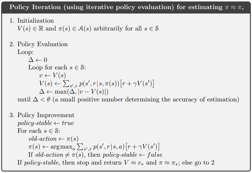Policy Iteration

Don’t worry, I will show you how to calcule the best policy using the yyxsb problem. 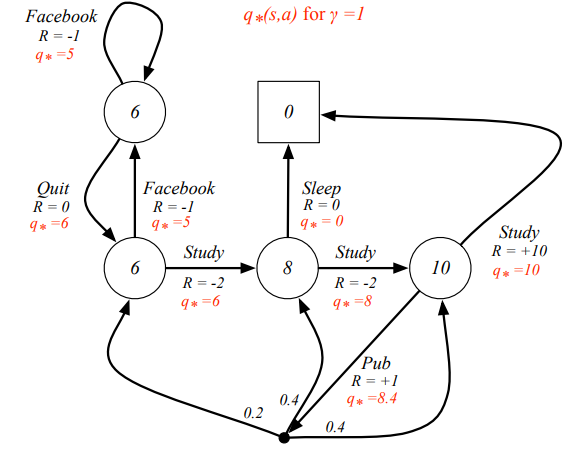yyxsb best state action value

Here I will show you how to calculate the $\pi_{*}$ using python.

import numpy as np
from copy import copy

gamma = 1.
def update_p_r(new_pi_list):
    P = np.matrix([[new_pi_list[0], 1 - new_pi_list[0], 0, 0, 0],
                   [new_pi_list[1], 0, 1 - new_pi_list[1], 0, 0],
                   [0, 0, 0, 1 - new_pi_list[2], new_pi_list[2]],
                   [0, 0.2 * new_pi_list[3], 0.4 * new_pi_list[3], 0.4 * new_pi_list[3], 1 - new_pi_list[3]],
                   [0, 0, 0, 0, 1]])
    R = np.matrix([new_pi_list[0]*(-1), new_pi_list[1] * (-1) + (1 - new_pi_list[1]) * (-2), (1 - new_pi_list[2])*(-2), new_pi_list[3] + (1 - new_pi_list[3]) *10, 0]).T
    return P ,R
	
def update_pi(P, R, V):
    pi_list = [0, 0, 0, 0, 0]
    for m in range(len(pi_list)):
        pi_list_0 = copy(pi_list)
        pi_list_0[m] = 0
        P, R = update_p_r(pi_list_0)
        V_a_0 = R + gamma * P * V
        
        pi_list_1 = copy(pi_list)
        pi_list_1[m] = 1
        P, R = update_p_r(pi_list_1)
        V_a_1 = R + gamma * P * V
        #print(V_a_0[m, 0], V_a_1[m, 0])
        #print("---")
        if V_a_0[m, 0] >= V_a_1[m, 0]:
           pi_list = pi_list_0
           #print("pi_list: ",pi_list)
        else:
           pi_list = pi_list_1
    return pi_list
		
stable_count = 0
pi_list = [0,1,0,1,0]
policy_stable = False
while policy_stable != True:

    # policy evaluation
    P, R = update_p_r(pi_list)
    V = np.matrix([0,0,0,0,0]).T
    for _ in range(5):
    	V = R + gamma * P * V
    #print(V)	
    # policy improvement
    #policy_stable = True
    old_pi_list = copy(pi_list)
    pi_list = update_pi(P, R, V)
    #print(pi_list)
    if pi_list == old_pi_list:
    	stable_count += 1
    	if stable_count >= 5 :
    		 policy_stable = True
    else:
    	stable_count = 0
    #break
	
print("best V: ", str(V))
print("best Pi: ", str(pi_list))
#print(Pi, P, R)
#print(V)

Value Iteration

One drawback to policy iteration is that each of its iterations involves policy evaluation. The question is: can’t we just find out the best value functions, then calculate $\pi_{*}$? Then anwser is yes. 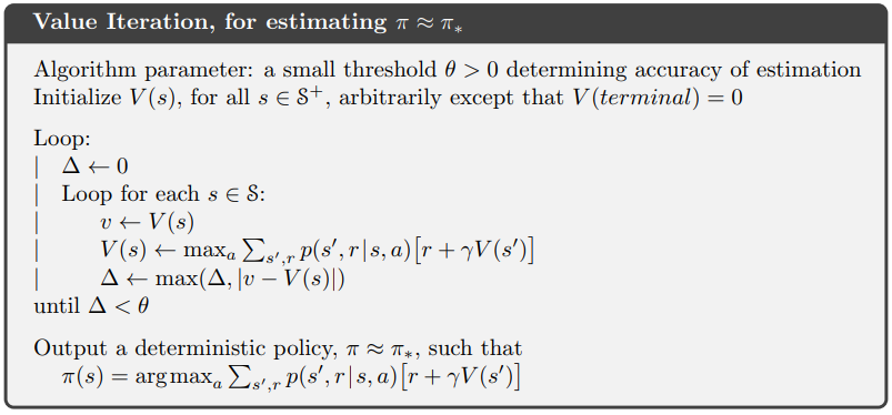Value Iteration

Here is the python code for the same problem.

import numpy as np
from copy import copy

gamma = 0.9
def get_p_r(new_pi_list):
    P = np.matrix([[new_pi_list[0], 1 - new_pi_list[0], 0, 0, 0],
                   [new_pi_list[1], 0, 1 - new_pi_list[1], 0, 0],
                   [0, 0, 0, 1 - new_pi_list[2], new_pi_list[2]],
                   [0, 0.2 * new_pi_list[3], 0.4 * new_pi_list[3], 0.4 * new_pi_list[3], 1 - new_pi_list[3]],
                   [0, 0, 0, 0, 1]])
    R = np.matrix([new_pi_list[0]*(-1), new_pi_list[1] * (-1) + (1 - new_pi_list[1]) * (-2), (1 - new_pi_list[2])*(-2), new_pi_list[3] + (1 - new_pi_list[3]) *10, 0]).T
    return P ,R
	
def update_v(V):
    pi_list = [0, 0, 0, 0, 0]
    V_new = np.matrix([0, 0, 0, 0, 0]).T
    for m in range(len(pi_list)):
        pi_list_0 = copy(pi_list)
        pi_list_0[m] = 0
        P, R = get_p_r(pi_list_0)
        V_a_0 = R + gamma * P * V
        
        pi_list_1 = copy(pi_list)
        pi_list_1[m] = 1
        P, R = get_p_r(pi_list_1)
        V_a_1 = R + gamma * P * V
        
        #print(V_a_0[m, 0], V_a_1[m, 0])
        #print("---")
        if V_a_0[m, 0] >= V_a_1[m, 0]:
            V_new[m,0] = V_a_0[m, 0]
        else:
            V_new[m,0] = V_a_1[m, 0]
    return V_new
	
	
def update_pi(V):
    pi_list = [0, 0, 0, 0, 0]
    for m in range(len(pi_list)):
        pi_list_0 = copy(pi_list)
        pi_list_0[m] = 0
        P, R = get_p_r(pi_list_0)
        V_a_0 = R + gamma * P * V
        
        pi_list_1 = copy(pi_list)
        pi_list_1[m] = 1
        P, R = get_p_r(pi_list_1)
        V_a_1 = R + gamma * P * V
        #print(V_a_0[m, 0], V_a_1[m, 0])
        #print("---")
        if V_a_0[m, 0] >= V_a_1[m, 0]:
            pi_list = pi_list_0
        else:
            pi_list = pi_list_1
    return pi_list
		
stable_count = 0
pi_list = [0,1,0,1,1]
theta = 0.001
V = np.matrix([10000, 200, 0, 0, 0]).T
stable = False
while stable == False:
    V_new = update_v(V)
    if (np.linalg.norm(V - V_new)) < theta:
        print("stable!")
        stable = True
    else:
        V = V_new
    #gprint(V)

pi_list = update_pi(V)
	
print("best V: ", str(V))
print("best Pi: ", str(pi_list))

What can we learn from DP? - Generalized Policy Iteration

Ok, every thing seems ok. We’ve shown the algorithm to use DP. But since the algorithm above is slow and with a lot of drawbacks like known model assumption, why we still need to learn it?

In fact, we can notice the algorithms above: First evaluate policy, then improve it. It becomes a generasized idea in reinforcement learning, which you will see them in the later posts. 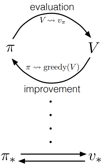Generalized Policy Iteration

The evaluation and improvement processes in GPI can be viewed as both competing and cooperating. They compete in the sense that they pull in opposing directions. Making the policy greedy with respect to the value function typically makes the value function incorrect for the changed policy, and making the value function consistent with the policy typically causes that policy no longer to be greedy. In the long run, however, these two processes interact to find a single joint solution: the optimal value function and an optimal policy. We will use this idea in the following posts.

Another important truth

As you have noticed, every time we update $V$ or $q$, the $V$ or $q$ becomes bigger! That means we are improving our policy. But, why? Here is the theorem.

Policy improvement theorem
Let $\pi$ and $\pi^{\prime}$ be any pair of deterministic policies such that, for all $s \in \mathcal{S}$, $q_{\pi}\left(s, \pi^{\prime}(s)\right) \geq v_{\pi}(s)$ Then the policy $\pi^{\prime}$ must be as good as, or better than $\pi$: $v_{\pi^{\prime}}(s) \geq v_{\pi}(s)$.

Here is the proof:

$\begin{array}{l}{v_{\pi}(s) \leq q_{\pi}(s, \pi^{\prime}(s)) } \\ {=\mathbb{E}\left[R_{t+1}+\gamma v_{\pi}\left(S_{t+1}\right) | S_{t}=s, A_{t}=\pi^{\prime}(s)\right]} \\ {=\mathbb{E}_{\pi^{\prime}}\left[R_{t+1}+\gamma v_{\pi}\left(S_{t+1}\right) | S_{t}=s\right]} \\ { \leq \mathbb{E}_{\pi^{\prime}}\left[R_{t+1}+\gamma q_{\pi}\left(S_{t+1}, \pi^{\prime}\left(S_{t+1}\right)\right) | S_{t}=s\right]} \\ {=\mathbb{E}_{\pi^{\prime}}\left[R_{t+1}+\gamma \mathbb{E}_{\pi^{\prime}}\left[R_{t+2}+\gamma v_{\pi}\left(S_{t+2}\right) | S_{t+1}, A_{t+1}=\pi^{\prime}\left(S_{t+1}\right)\right] | S_{t}=s\right]} \\ {=\mathbb{E}_{\pi^{\prime}}\left[R_{t+1}+\gamma R_{t+2}+\gamma^{2} v_{\pi}\left(S_{t+2}\right) | S_{t}=s\right]} \\ { \leq \mathbb{E}_{\pi^{\prime}}\left[R_{t+1}+\gamma R_{t+2}+\gamma^{2} R_{t+3} + \gamma^{3}v_{\pi}(S_{t+3}) | S_{t}=s\right]} \\ {\vdots} \\ {\leq \mathbb{E}_{\pi^{\prime}}\left[R_{t+1}+\gamma R_{t+2}+\gamma^{2} R_{t+3}+\gamma^{3} R_{t+4} + \ldots | S_{t}=s\right]} \\ { = v_{\pi^{\prime}}(s)}\end{array}$

Summary

In this post, I’ve showed you how to understand DP easily through algorithms and codes. However, we will never use DP in real life, why? Please check this post: An Easy Way To Understand Monte Carlo Learning In Reinforcement Learning.

References

• David Silver-Dynamic Programming
• Reinforcement Learning Demystified: Solving MDPs with Dynamic Programming

---

You May Also Enjoy

A Least Squares Approach --Math

Linear Modeling - A Maximum Likelihood Approach --Math

The Bayesian Approach To Machine Learning --Math

An Introduction To ESN --Math

Modeling With NMF And SVD --Math

Bounding Box Regression --Math

Welcome to share or comment on this post: