An Easy Way To Understand Monte Carlo Learning In Reinforcement Learning

---

Introduction

We all hope that robot can learn from experiences by interacting with environment itself, and Monte Carlo (MC) is an important way to achieve this. In the last post, we’ve introduced that dynamic learning can be used to find the optimal policy for a system, however, in real world applications, we often don’t know complete knowledge about environment, which means DP will be never used. But Monte Carlo learning don’t require any prior knowledge about the environment dynamics, yet can still attain optimal behavior.

In this post, I will show you how and why MC works with minimal math knowledge.

What is Monte Carlo learning - Intuition?

Imagine, our stupid friend yyxsb is playing an atari game, and he want to clear that game. But unfortunately, he is stupid thus he have to try many times to find all the traps and avoid the enemy to improve his ability, say 100,000 times for a simple game. Every time he play a round, we remember the time series data like state:(position, life …), action:(left or right), reward:(say 1). Then we can collect 100,000 episodes. For simplicity, we assume the game has only 10 scenes (states).

We found yyxsb is too stupid to complete that game beutifully, then we decide to invent a robot to help him complete that game easily. Fortunately, he gave us 100,000 episodes of data and we can do something with it!

So the next question is: How to train a robot from those ugly generated episodes? In fact, for every scene (state), we can estimate wether its good or not, then determine next action, right? That’s it, yyxsb does the same thing, also, our robot need to try it. For every episode, the robot can learn whether the scene (state) is good or not, then change it’s policy. We call this process learning. After learning all the episodes, our robot is invincible, of course better than stupid yyxsb. That’s Monte Carlo learning: learning from experience. Or off-policy Monte Carlo learning.

Remember that in the last post - dynamic programming, we’ve mentioned generalized policy iteration (GPI) is the common way to solve reinforcement learning, which means first we should evaluate the policy, then improve policy. In Monte Carlo learning, we do exactly the same things. The difference is that we use experience to evaluate the policy. If you don’t understand what are policy and state value, you should first read this post first.

What? You still cannot get what’s MC? Don’t worry, I will tell you the details now.

Why do we need to introduce Monte Carlo learning?

We are living in a world that is full of data, however, we don’t know the details of environment that generated that data. Thus it’s natural for us that the machine can learn from interaction with environment.

Since we don’t have prior knowledge about environment, which means we cannot calculate the state value, let alone policy. But we have a lot of data. Monte Carlo learning provides a data based learning method by averaging sampled returns, which is practical.

How to understand Monte Carlo learning?

How to estimate state values?

This is the first problem we need to solve, right? Without state value, we cannot even sleep well. In fact it is very easy. We just average the return for every time a state appears in every episode, or average the return for the first time a state appears in every episode! If we have infinite episodes, then the average return for every state is mean return (which is expect to equal to expect return)! That’s MC, just average, no special.

But, sometimes you will find that some states will never happen in a game, but it’s also very important, we need to find a way!
In here, two methods:

• Exploring starts. We just ensure that our episodes include all states.

• Non-deterministic policy. We just let the policy non-deterministic. I mean, for all state, $\pi(s) > 0$. Then all states may be explored. This will be the main part of this post.

We use these two methods to collect episodes.

Just show me tho algorithm:
Updata $V_{s}$ incrementally after an episode $S_{1}, A_{1}, R_{1}, \ldots, S_{T}$
For each state $S_{t}$ with return $G_{t}$(we get $G_{t}$ by iterating episode inversely) $\begin{array}{l}{N\left(S_{t}\right) \leftarrow N\left(S_{t}\right)+1} \\ {V\left(S_{t}\right) \leftarrow V\left(S_{t}\right)+\frac{1}{N\left(S_{t}\right)}\left(G_{t}-V\left(S_{t}\right)\right)}\end{array}$

$N$ in algorithm above means appear numbers for each state.

Here is the proof for the algrithem above.
$v(s) = \frac{1}{k} \sum_{j=1}^{k}G_{j}(s)$ $= \frac{1}{k}\Bigg(G_{k}(s) + \sum_{j=1}^{k-1}G_{j}(s) \Bigg)$ $= \frac{1}{k}(G_{k}(s) + (k-1)v_{k-1}(s) )$ $= v_{k-1}(s) + \frac{1}{k}(G_{k}(s) - v_{k-1}(s))$

Notice that $G$ is calculated from episode, while in DP, $G$ is calculated from known parameter.

I think you’ve familar with $V(s)$, but in fact $q(s,a)$ is almost the same, but easier to calculate in real applications, so I will try to use more $q(s, a)$ in later description.

How to get optimal policy?

Greedy! Like this: $\pi(s) \doteq \arg \max _{a} q(s, a)$

Easy, right? Here is the algorithm for all the process. 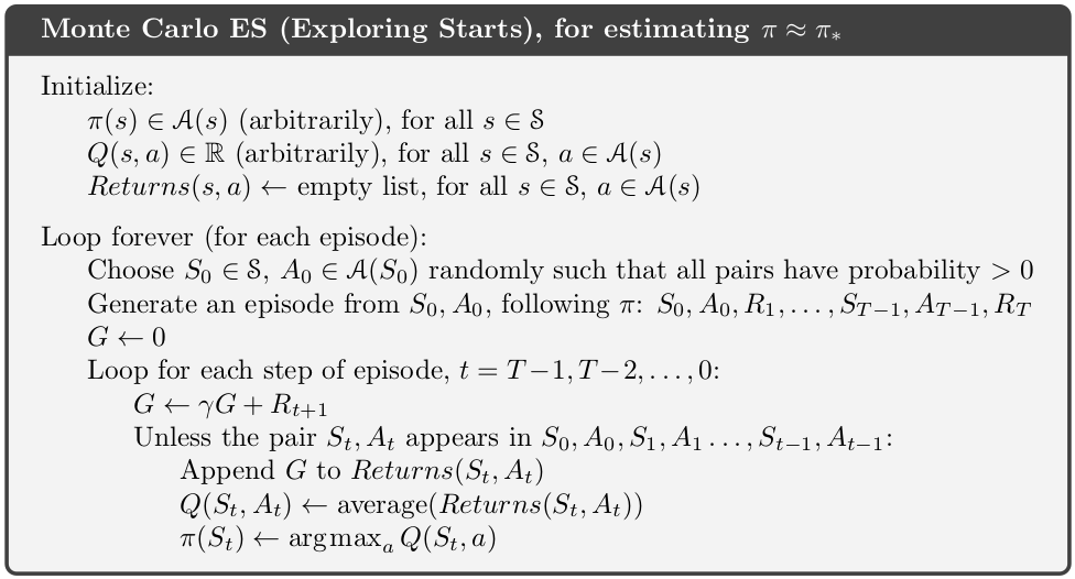Monte Carlo Exploring Starts for estimating $\pi_{*}$

The reason we calculate the mean return $G$ from back to start is: $G_{t} = 0, t = T$. Thus we can get all mean return via iteration.

Here is why we can get optimal policy: $\begin{aligned} q_{\pi_{k}}\left(s, \pi_{k+1}(s)\right) &=q_{\pi_{k}}\left(s, \arg \max _{a} q_{\pi_{k}}(s, a)\right) \\ &=\max _{a} q_{\pi_{k}}(s, a) \\ & \geq q_{\pi_{k}}\left(s, \pi_{k}(s)\right) \\ & \geq v_{\pi_{k}}(s) \end{aligned}$ According to policy improvement theorem, MC control can converge to optimal.

From here we talk about real MC

What! I’m not joking. Characters above is almost useless in practice, just to show you how MC works. I will tell you why.

In fact, the MC we talked above has an important assumption: exploring starts, to ensure the robot can explore all states. But in real world applications, that’s impossible, since we usually cannot determine the initial state. For example, can you determine your money, rank and birth place in a RPG game start?

Thus to ensure exploring all states, we need to make policy non-deterministic to collect data.

Depending on if the data collecting policy is the same to targeting policy (the policy we want to improve), we divide them into on-policy (the same), and off-policy (not the same. Remember yyxsb play game? Since yyxsb has different policy from robot, it’s off-policy)

How to use on-policy MC learning?

In fact, it’s still very easy, the algorithm is: 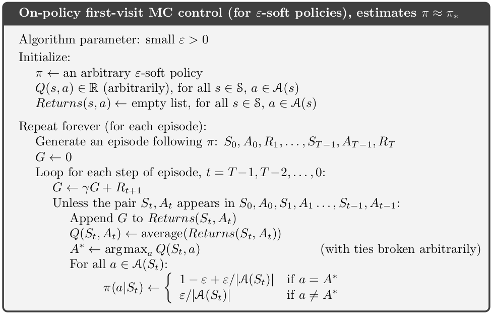On-policy first-visit MC control for estimating $\pi_{*}$

Here we use the same $\varepsilon$-greedy policy to collect episode and optimize.

You will notice that the algorithm use state action value instead. Why? In fact, state value is not sufficient to determine policy if we don’t know the model of the environment. But state action value can determine a policy.

Also, I have to state that for all MC updates, it completely updates the $V$ or $Q$ after a complete episode.

How to use off-policy MC learning?

It’s the key part of this post. Since off-policy is very promising, we have to talk about it in detail. Off-policy is really cool, since robot can learn from data that generated from others!

So the new question is: how to get the target policy from a known data generate policy? In fact, there are many ways like:

• …

• importance sampling

• MCMC

In this post, I will only show you method based on importance sampling.

About how to improve importance sampling and the python code, please refer to this post: Importance Sampling In Reinforcement learning

With importance sampling, we can calculate the average state action value from data generated by another known distribution. However, in real world application, we often want or have to calculate $q(s, a)$ incrementally. Suppose we have a sequence of returns $G_{1}, G_{2}, \ldots, G_{n-1}$, all starting in the same state and each with a corresponding random weight $W_{i}$. From importance sampling, we know that we need to estimate $V_{n} \doteq \frac{\sum_{k=1}^{n-1} W_{k} G_{k}}{\sum_{k=1}^{n-1} W_{k}}, \quad n \geq 2$ equals to $\frac{\sum_{k}^{n} W_{k} G_{k}+W_{n+1} G_{n+1}}{\sum_{k}^{n} W_{k}} \frac{\sum_{k}^{n} W_{k}}{\sum_{k}^{n+1} W_{k}}$ $=V_{n} \frac{C_{n-1}}{C_{n}}+W_{n} \frac{G_{n}}{C_{n}}$ $\begin{array}{l}{=V_{n}+\frac{W_{n} G_{n}-V_{n} W_{n}}{C_{n}}} \\ {=V_{n}+\frac{W_{n}}{C_{n}}\left(G_{n}-V_{n}\right)}\end{array}$ and $C_{n+1} \doteq C_{n}+W_{n+1}, C_{0} \doteq 0$

We can exchange $V$ to $Q$ without worry, and $C_{n}$ is cumulative sum of the weights. Here is the algorithm. 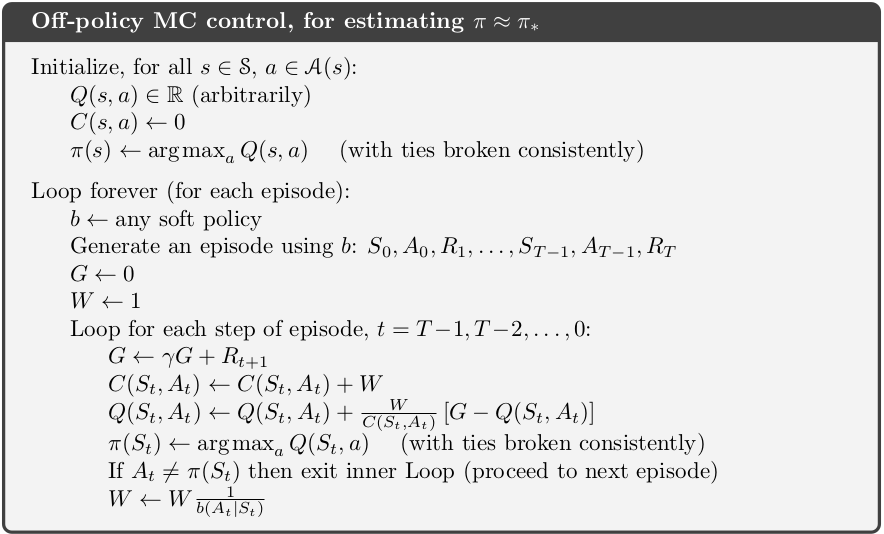Off-policy MC control for estimating $\pi_{*}$

What? you may have been expecting the $W$ update to have involved the importance-sampling ratio $\frac{\pi\left(A_{t} | S_{t}\right)}{b\left(A_{t} | S_{t}\right)}$ from this post that introduced importance sampling, but instead it involves $\frac{1}{b\left(A_{t} | S_{t}\right)}$. Why is this nevertheless correct? In fact, when $W = 0$, we need to stop that route since we don’t need to learn from that epison any more (don’t need to learn bad ideas from episode, that’s why the policy can become better), and $\pi(A_{t}|S_{t}) = 0/1$, thus we can use $\frac{1}{b\left(A_{t} | S_{t}\right)}$ instead.

Drawbacks of MC learning

As you can see, we have to wait the whole episode ends to update $Q,\pi$ for all states, which makes MC learning super slow if an episode is very long, like, a round of LOL. Another important drawback is that some MC methods must ignore or discount episodes on which experimental actions are taken (like: not the same to actions for off-policy learning), which can greatly slow learning. So any ways to solve this problem? Of course, I will show you in the next post.

Summary

In this post, we’ve explored why and how MC learning works. MC learning is very important in real world applications, however, since it’s very slow, we don’t use MC directly.

References

• David Silver-Model-Free Prediction
• Reinforcement Learning: An Introduction - MC learning
• Monte Carlo in Reinforcement Learning, the Easy Way
• Reinforcement Learning: Introduction to Monte Carlo Learning using the OpenAI Gym Toolkit

---

You May Also Enjoy

A Least Squares Approach --Math

Linear Modeling - A Maximum Likelihood Approach --Math

The Bayesian Approach To Machine Learning --Math

An Introduction To ESN --Math

Modeling With NMF And SVD --Math

Bounding Box Regression --Math

Welcome to share or comment on this post: