An Easy Way To Understand Markov Decision Process In Reinforcement Learning

---

Introduction

If you can’t explain it simply, you don’t understand it well enough.     - - Albert Einstein

Markow Decision Process (MDP) is very useful in modeling sequential decision making problems like video games (atari, starcraft etc.) or chatbot systems. In this post, I will give you a detail description on how markov decision process describes reinforcement learning problems with only high school level math, and I hope this post provide basic knowledge for deeper understanding MDP.

Why MDP is introduced?

Imagine, our friend yyxsb, want to live a richer life in 4 years later. He will make a big decision every year and implement that decision that whole year. For simplicity, we assume that he has only two options: work and play. To get richer, he have to work harder, haha.

Thus we know, yyxsb has T=4 decisions to make. Which will lead to 2*2*2*2=16 different decision chains. For example:

C1 = [play, play, play, play]
C2 = [play, work, work, work]
C3 =[work, play, work, play]
…

If you don’t work you don’t eat. yyxsb want to save money in the long run, but play will cost a lot. In here, we assume the reward of working a year is $10k, and playing a year costs $8k. That is [10k, -8k] for the rewards responding to actions [work, play]. We assume that he can be in debt, so 4 years the money yybsb can own is between [-8k*4, 10k*4] = [-32k, 40k].

Every year yyxsb can make a new decision according to money he has now. In here we give a example of how he make decisions.

state0: {money: 0k, year: 0}, action0: play ->
reward1: -8k, state1: {money: -8k, year: 1}, action1: play ->
reward2: -8k, state2: {money: -16k, year: 2}, action2: play ->
reward3: -8k, state3: {money: -24k, year: 3}, action3: play ->
reward4: -8k, state4: {money: -32k, year: 4}

At this decision chain, in the end of 4th year, he has -32k. But in fact there are 16 different decision chains like that. We may often want to know how yyxsb will make decision in this process with rewards to get most final reward. In fact this example is a mini markov decision process: in state, take action, get reward.

Generally, for better compute the final reward of a process like make money or play video games, we can use a powerful tool – markov decision process to describe it. Why? because the math property of MDP make it perfect to model sequential decision process.

How to understand MDP for modeling sequential decision making problems?

Assumption

The future is independent of the past given the present

A formal description:
A state $S_{t}$ is Markov if and only if $\mathbb{P}\left[S_{t+1} | S_{t}\right]=\mathbb{P}\left[S_{t+1} | S_{1}, \ldots, S_{t}\right]$ $S_{t}$ in here means state in time $t$. Take the yyxsb’s 4 year goal as example, if the third year’s state is only depend on the second year’s state, then the process is markov process.

A gentle description to MDP

First I have to strees here that our goal is to understand how MDP works. MDP: markov decision process, but to understand it, we first introduce markov process.

Markov process

Imagine again, yyxsb is enjoying his university life, like this: 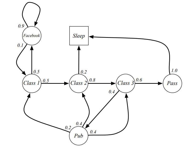yyxsb markov chain

The number in the picture represent probobility of transferring from one state to another. For example, when you are checking facebook, you still have $p = 0.9$ probability to continue it in one hour later. Since a day will over, often the last state of a decision chain of yyxsb is sleep, thus the example chains like:

• C1 C2 C3 Pass Sleep
• FB FB FB C1 C2 Sleep
• C1 C2 C3 Pub C2 C3 Pass Sleep

In this example, it can be infinite because loops exist like check facebook. To describe the possibility of transfer from one state to another state in a formal way, we have:

• State Transition Probability: The state transition probability tell us, given we are in state $s$ what the probability the next state $s^{\prime}$ will occur. $\mathcal{P}_{s s^{\prime}}=\mathbb{P}\left[S_{t+1}=s^{\prime} | S_{t}=s\right]$

Then we can define a matrix to show to whole probability in a mathimatical way. Why? It’s easy to compute for computers. $\mathcal{P}=\text { from }\left[\begin{array}{ccc}{\mathcal{P}_{11}} & {\stackrel{t o}{\ldots}} & {\mathcal{P}_{1 n}} \\ {\vdots} & {} & {} \\ {\mathcal{P}_{n 1}} & {\cdots} & {\mathcal{P}_{n n}}\end{array}\right]$

for yyxsb’s university life example, the state transition matrix is: State Transition Matirx

We can see that probability of transfering from facebook to facebook is $p(FB|FB) = 0.9$ (When state now is $FB$, the probability of next state = $FB$).

Then we can know: markov process is a process that consist of $S$(a set of states) and $P$(state transition probability matrix). Marked as $<S, P>$

Stop, don’t be puzzled about it. Why we need to understand the descriptions above? Still remember yyxsb’s 4 year goal example? isn’t them similar? Yes, if we add a decision part for markov process, then it becomes markov decision process.

However, to make a decision, we need a judge criteria, otherwise we don’t know which decision is better, isn’t it?

Reward

For yyxsb, money is everything, unlike that, we need a general definition, in here, we use reward:

• Reward: The reward $Rₜ$ is a scalar feedback signal which indicates how well the agent is doing at step time t.

Not so easy to understand, but don’t worry, just think it as: the reward you get when you finished a work.

The next problem is: How to describe an average reward for a specific state? If we know this value, then we can always choose the best state, looks good, isn’t it? Since it’s a general needs, we define a reward function here We define the reward function as: $\mathcal{R}_{s}=\mathbb{E}\left[R_{t+1} | S_{t}=s\right]$ For a state, there may exist many following states with different rewards

The next problem is: How to describe the total return for a specific time $t$? If we know the total return, then it can help use to make decisions. For example, we can calculate the total return is $ $40k$ when yyxsb choose only work for the beginning. Thus we introduce an useful variable $G_{t}$: $G_{t}=R_{t+1}+\gamma R_{t+2}+\ldots=\sum_{k=0}^{\infty} \gamma^{k} R_{t+k+1}$

First let’s assume $\gamma = 0$, that means, we think total future reward is next step’s reward. For example, we choose to play games instead of read books because the inmidiate reward of play games is bigger than read books. But we know, in a long-term perspective, by reading books we can get more. That means: for the guys choose $\gamma = 0$, they are “short-sighted”, also, we don’t often choose $\gamma = 0$ in reinforcement learning.

How about $\gamma = 1$? Well, unlike $\gamma = 0$, this will lead to “far-sighted” result. Is this better? Unfortunately no, because time is limited, we cannot expect for the money we get surprisely after we died.

Thus it’s obvious that we should choose $\gamma$ between $0$ and $1$. It means the reward from far future is not so important, we use $\gamma$ as a decay factor. There are also other reasons:

• Mathematically convenient to discount rewards
• Avoid infinite returns in cyclic markov process
• Uncertainty about the future may not be fully represented
• Sometimes impossible to use $\gamma = 1$

Like this figure, the reward means transfer from state A to state B, we can get that reward. 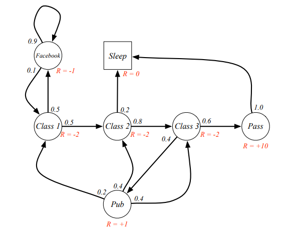yyxsb reward process

Thus we can calculate the long-term expect return for state $s$! Why it is important? Because it helps us to make decisions, for example, we can calculate the total return is $ $40k$ when yyxsb choose only work for the beginning. You must have laugh at me that I use such a stupid example, but think it over again: we first calulate the expect value for making different decision, then find out the best is to choose work all the time, right? That’s it! In reinforcement learing, we calculate expect return to help us make decisions! We define it as state value fuction $v(s)$ $v(s)=\mathbb{E}\left[G_{t} | S_{t}=s\right] \tag{1}$

For example, expect return from yyxsb’s university life markov process:
Starting from $S_{1} = C1$ with $\gamma = 1/2$ $G_{1}=R_{2}+\gamma R_{3}+\ldots+\gamma^{T-2} R_{T} \tag{2}$

For different possible chains of the same state like $S_{1}$, there may exist many values. For the above figure, we have:

• C1 C2 C3 Pass Sleep $v_{1} = -2 -2*\frac{1}{2} - 4*\frac{1}{4} + 10 * \frac{1}{8} = -2.25$
• C1 FB FB C1 C2 Sleep $v_{1} = -2 -1 * \frac{1}{2} - 1 * \frac{1}{4} - 2 * \frac{1}{8} - 2 * \frac{1}{16} = -3.125$
• …

Wait! if there are many expect returns for a state, which one is state value function for that state? In fact, here we need to understand a important definition: state value fuction means expect value of $G_{t}$, given state $s$, however, in the example above, we’ve determined the process chain, thus the reward is fixed. Then for every chain, there is a specific expect return.

But what we want is an averaged expect return for a state, isn’t it? In fact we need to calculate all possible routes and average them, and that’s very troublesome, and usually we don’t calculate them directly. Don’t kick me, I will show you how to get the average state value. Here is the source code about how to calculate $v(s)$ in python.

import numpy as np

# translation matrix
P = np.array([[0. , 0.5, 0. , 0. , 0. , 0.5, 0. ],
              [0. , 0. , 0.8, 0. , 0. , 0. , 0.2],
              [0. , 0. , 0. , 0.6, 0.4, 0. , 0. ],
              [0. , 0. , 0. , 0. , 0. , 0. , 1. ],
              [0.2, 0.4, 0.4, 0. , 0. , 0. , 0. ],
              [0.1, 0. , 0. , 0. , 0. , 0.9, 0. ],
              [0. , 0. , 0. , 0. , 0. , 0. , 1. ]])
# reward vector
R = np.array([-2, -2, -2, 10, 1, -1, 0])

iterate = R
gamma = 0.9

# state value initialization
V = R
for _ in range(100):
    iterate = gamma * P@iterate
    V = V + iterate
print("state values are: ", str(V))

Result for $gamma = 0.9$:
[-5.012728 0.9426554 4.08702136 10. 1.90839263 -7.6376068 0. ]

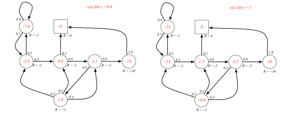yyxsb state value example

Here are some questions need to anwser:

1. What’s the formula to calculate the final state value?
   • Remember the formalat $(1)$ and $(2)$, that means we can calculate expect reward for every possible time, which is: $v(s)=\mathbb{E}\left[R_{2} + \gamma R_{3} + ... + \gamma^{T-2} R_{T} | S_{t}=s\right]$ We know $R_{2} = R = [-2, -2, -2, 10, 1, -1, 0]$, but how to calculate $\mathbb{E}[\gamma R_{3} + ...]$?
     $\mathbb{E}[R_{3}]$ means the second expect reward, we can use $P^{2}$ to show the possibility, then matrix multiply to $R$, we can get $\mathbb{E}[R_{3}] = P^2 \times R$, the same to others. $v(s) = R + \gamma P\times R + \gamma^{2} P^2\times R + ...$
2. Why we need to iterate 100 times to get the final result?
   • As we increase iterate numbers, the result will not change at all. $P^{100} \approx P^{1000000}$
3. Why we dont’ use this formula in real-world application?
   • You can see the computational complexity is $O(m n^3), m = 100, n = 7$ here. As $n$(state number) arises, it’s difficult to calculate.

So we need a better method to calculate state value, which leads to bellman equations.

Bellman Equations

In here I will show you how to get an averaged expect return.

From definition, we have: $\begin{aligned} v(s) &=\mathbb{E}\left[G_{t} | S_{t}=s\right] \\ &=\mathbb{E}\left[R_{t+1}+\gamma R_{t+2}+\gamma^{2} R_{t+3}+\ldots | S_{t}=s\right] \\ &=\mathbb{E}\left[R_{t+1}+\gamma\left(R_{t+2}+\gamma R_{t+3}+\ldots\right) | S_{t}=s\right] \\ &=\mathbb{E}\left[R_{t+1}+\gamma G_{t+1} | S_{t}=s\right] \\ &=\mathbb{E}\left[R_{t+1}+\gamma v\left(S_{t+1}\right) | S_{t}=s\right] \tag{3} \end{aligned}$

That is immediate reward $R_{t+1}$ and discounted value of successor state $\gamma v(S_{t+1})$, you can see it here, we need to calculate the next state’s expect value to get $v(s)$.

From the formula $(3)$ we can get $v(s)=\mathcal{R}_{s}+\gamma \sum_{s^{\prime} \in \mathcal{S}} \mathcal{P}_{s s^{\prime}} v\left(s^{\prime}\right \tag{4})$ Which is the same formula we got above. Show it in graph: 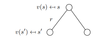State value relationship

In fact, we can also express formula $(4)$ more concisely using matrices: $\begin{aligned} v &=\mathcal{R}+\gamma \mathcal{P} v \\(I-\gamma \mathcal{P}) &=\mathcal{R} \\ v &=(I-\gamma \mathcal{P})^{-1} \mathcal{R} \end{aligned}$

Here is the code to test the result:

import numpy as np

# translation matrix
P = np.matrix([[0. , 0.5, 0. , 0. , 0. , 0.5, 0. ],
              [0. , 0. , 0.8, 0. , 0. , 0. , 0.2],
              [0. , 0. , 0. , 0.6, 0.4, 0. , 0. ],
              [0. , 0. , 0. , 0. , 0. , 0. , 1. ],
              [0.2, 0.4, 0.4, 0. , 0. , 0. , 0. ],
              [0.1, 0. , 0. , 0. , 0. , 0.9, 0. ],
              [0. , 0. , 0. , 0. , 0. , 0. , 1. ]])
# reward vector
R = np.array([-2, -2, -2, 10, 1, -1, 0])

iterate = R
gamma = 0.9

V = (np.identity(P.shape[0]) - gamma * P).I @ R
print("state values are: ", str(V))

Result for $gamma = 0.9$, which is the same to the result above:
[-5.01272891 0.9426553 4.08702125 10. 1.90839235 -7.63760843 0. ]

So is bellman equation the final solution to solve state value? Naive, of course not. Here is the reason:

• Computational complexity for $(4)$ is $O(n^{3})$ for n states
• Direct solution only possible for small markov process.
• Other iterative methods are better for large markov process.
  • Dynamic programming
  • Monte-Carlo evaluation
  • Temporal-Difference learning

So untill now, we understand how to calculate state value to help us make decisions, but we didn’t talked any thing about how to make decision! I’m not kidding you, markov process + action and reward = markov decision process.
I’m going to introduce Markov Decision Process now, to model the real world process.

Markov Decision Process

In a word, it’s a tuple $<\mathcal{S}, \mathcal{A}, \mathcal{P}, \mathcal{R}, \gamma>$

• $\mathcal{S}$ is a finite set of states
• $\mathcal{A}$ is a finite set of actions
• $\mathcal{P}$ is a state transition probability matrix, $\mathcal{P}_{s s^{\prime}}^{a}=\mathbb{P}\left[S_{t+1}=s^{\prime} | S_{t}=s, A_{t}=a\right]$
• $\mathcal{R}$ is a reward function, $\mathcal{R}_{s}^{a}=\mathbb{E}\left[R_{t+1} | S_{t}=s, A_{t}=a\right]$
• $\gamma$ is a discount factor $\gamma \in[0,1]$

Black dot in the figue means action note, and have possibilities turn to different state. Is it possible? see a rotot, in low battery, it can be broken or still work in the next state, right?
The figure means from a state, take an action then get a reward, turn to a new state, that’s all of MDP. 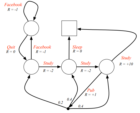yyxsb MDP

So, how to make decisions? Of course we need a robot or an algorithm to help us, right? In reinforcement learning, we call that amazong robot/algorithm - policy.

• Policy $\pi$ is a distribution over actions given states. $\pi(a | s)=\mathbb{P}\left[A_{t}=a | S_{t}=s\right]$
  • policy only depend on current state

Policy can tell us the posibilities of all actions, we can choose the biggest one as the next action. It’s over!

What? Such a easy formula can tell us which decision is better?

Simplicity is the ultimate sophistication     - - Da Vinci

Yes, the ultimate goal of reinforcement learning is to find a policy $\pi$ which returs an action help us to make decisions. Since I still haven’t introduce how to realize policy $\pi$ in computer programs, you can think it as a smart version of yyxsb (our great actor and friend, don’t forget him!), that he can make decisions from data, running on computers.

Thus, from now on, we need to add a limitations to all formula: given policy $\pi$. We can easily get

$\mathcal{P}_{s, s^{\prime}}^{\pi}=\sum_{a \in \mathcal{A}} \pi(a | s) \mathcal{P}_{s s^{\prime}}^{a} \tag{5}$ $\mathcal{R}_{s}^{\pi}=\sum_{a \in \mathcal{A}} \pi(a | s) \mathcal{R}_{s}^{a} \tag{6}$

Also the state-value function $v_{\pi}(s)$: $v_{\pi}(s)=\mathbb{E}_{\pi}\left[G_{t} | S_{t}=s\right]$

From the discussion above, we see the state-value function is in fact an expect return for all actions, but we also need to know the expect return with a action. Why? For example, yyxsb have no money, and choose to play this year, what the expect final result will be?
Then we introduce action value function $q_{\pi}(s,a)$, which is the expected return starting from state $s$, taking action $a$, and then following policy $\pi$ $q_{\pi}(s, a)=\mathbb{E}_{\pi}\left[G_{t} | S_{t}=s, A_{t}=a\right]$

From definition above, we know: $v_{\pi}(s)=\sum_{a \in \mathcal{A}} \pi(a | s) q_{\pi}(s, a) \tag{7}$

Here is a little difficult, pay attention, please. We need to find the relationship from $v_{\pi}(s)$ to $v_{\pi}(s^{\prime})$ and $q_{\pi}(s,a)$ to $q_{\pi}(s^{\prime},a^{\prime})$, which you can see that it helps to help us to calculate state value or action value, to find out optimal policy. In fact, from $(7)$ we can see, state-action pairs or action value functions are part of state value function. They are both expect return, just in different condition. In graph format, that’s 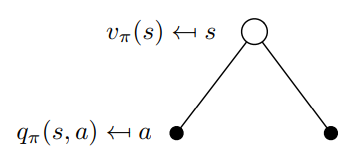Relationship between state value function and action value function

We can prove $v_{\pi}(s)=\sum_{a \in \mathcal{A}} \pi(a | s)\left(\mathcal{R}_{s}^{a}+\gamma \sum_{s^{\prime} \in \mathcal{S}} \mathcal{P}_{s s^{\prime}}^{a} v_{\pi}\left(s^{\prime}\right)\right) \tag{8}$ from Bellman Equation V(s) Proof. You see what? Yes equation $(7)$, that means: $q_{\pi}(s, a)=\mathcal{R}_{s}^{a}+\gamma \sum_{s^{\prime} \in \mathcal{S}} \mathcal{P}_{s s^{\prime}}^{a} v_{\pi}\left(s^{\prime}\right) \tag{9}$ and $q_{\pi}(s, a)=\mathcal{R}_{s}^{a}+\gamma \sum_{s^{\prime} \in \mathcal{S}} \mathcal{P}_{s s^{\prime}}^{a} \sum_{a^{\prime} \in \mathcal{A}} \pi\left(a^{\prime} | s^{\prime}\right) q_{\pi}\left(s^{\prime}, a^{\prime}\right) \tag{10}$ In graph format: 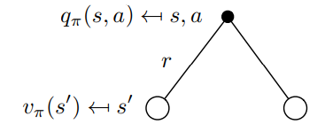Relationship between action value function and next state value function

From the above formula, we could get: 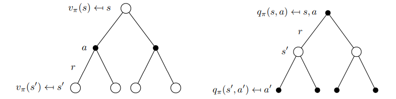State value function and action value function

Ok, don’t be panic! That’s not so difficult, it’s just, very troublesome. See the figure left above. We have a state, then have $\pi(a|s)$ possibility make decision to take action $a$, here it becomes an state-action pairs as mentioned (even if you take actions, you don’t go to a sure state sometimes, like a robot.), then go to different state, get a reward, that’s it. Also, in the right figure, start from a state-action pair, get a reward to a new state, then take new action to a new state-action pair. You can see figure left is easier to understand, right?

Let’s check if formula $(8)$ is righ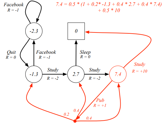t. yyxsb state value calculate

We can also express the formula in matrix format: $v_{\pi}=\mathcal{R}^{\pi}+\gamma \mathcal{P}^{\pi} v_{\pi}$ $v_{\pi}=\left(I-\gamma \mathcal{P}^{\pi}\right)^{-1} \mathcal{R}^{\pi} \tag{11}$

From $(5),(6)$, we can calculate $\mathcal{P}^{\pi}$ and $\mathcal{R}^{\pi}$: $\mathcal{P}^{\pi}: \left[\begin{array}{lllll}{0.5} & {0.5} & {0} & {0} & {0} \\{0.5} & {0} & {0.5} & {0} & {0} \\ {0}& {0} & {0} & {0.5} & {0.5} \\ {0} & {0.1} & {0.2} & {0.2} & {0.5} \\ {0}&{0}&{0}&{0}&{1} \end{array}\right]$

$\mathcal{R}^{\pi}: \left[\begin{array}{lllll}{-0.5} & {-1.5} & {-1} & {5.5} & {0} \end{array}\right]^{T}$

The order responding to states above is: $[-2.3, -1.3, 2.7, 7.4, 0]$. Here I will show you how to calculate state $7.4$ for $\mathcal{P}^{\pi}$ and $\mathcal{R}^{\pi}$:

• For $\mathcal{P}^{\pi}$, that’s the fourth row of $\mathcal{P}^{\pi}$ matrix. $P = 0.5$ for study, $P = 0.5 * 0.2$ for state $-1.3$, and so on.
• For $\mathcal{R}^{\pi}$, that’s the fourth number: $5.5$, which is $1*0.5 + 10 * 0.5$.

Then I will show two different method to calculate all the state value:

# Method one
import numpy as np

# translation matrix
P = np.matrix([[0.5, 0.5, 0. , 0. , 0. ],
            [0.5, 0. , 0.5, 0. , 0. ],
            [0. , 0. , 0. , 0.5, 0.5],
            [0. , 0.1, 0.2, 0.2, 0.5],
            [0. , 0. , 0. , 0. , 1. ]])

# reward vector
R = np.matrix([[-0.5, -1.5, -1. ,  5.5,  0. ]]).T

iterate = R
gamma = 1.0

# state value initialization
V = R
for _ in range(100):
    iterate = gamma * P@iterate
    V = V + iterate
print("state values are: ", str(V))

Result for $gamma = 1$:
[-2.30769231, -1.30769231, 2.69230769, 7.38461538, 0. ]

Or through $(11)$

# Method two
import numpy as np
# translation matrix
P = np.matrix([[0.5, 0.5, 0. , 0. , 0. ],
            [0.5, 0. , 0.5, 0. , 0. ],
            [0. , 0. , 0. , 0.5, 0.5],
            [0. , 0.1, 0.2, 0.2, 0.5],
            [0. , 0. , 0. , 0. , 1. ]])

# reward vector
R = np.matrix([[-0.5, -1.5, -1. ,  5.5,  0. ]]).T

iterate = R
gamma = 0.999

V = (np.identity(P.shape[0]) - gamma * P).I @ R
print("state values are: ", str(V))

Result for $gamma = 0.999$, which is almost the same to the result above:
[-2.30657961, -1.31019639, 2.68656682, 7.38051416, 0. ]

Question: why do I choose $gamma = 0.999$ in above program? In fact, sometimes the inverse matrix maybe singular, so…

Great! Till now, we know how to express MDP in pure math format, and we understand how to calculate state value functions. But we still don’t know how to choose policy $\pi$, don’t worry, I will show you now.

Optimal Value Function

Remember the yyxsb’s 4 year goal? We know that if he choose to work all the time, he can get a lot of money, because we’ve calculated the value for him. In reinforcement learning, we also need to find optimal value to determine the policy. An MDP is solved when we know the optimal value function. Here are the definitions: $v_{*}(s)=\max _{\pi} v_{\pi}(s)$ $q_{*}(s, a)=\max _{\pi} q_{\pi}(s, a)$ Easy, right? For $v_{*}(s), \gamma = 1$: $\mathcal{P}^{\pi}: \left[\begin{array}{lllll}{0} & {1} & {0} & {0} & {0} \\{0} & {0} & {1} & {0} & {0} \\ {0}& {0} & {0} & {1} & {0} \\ {0} & {0} & {0} & {0} & {1} \\ {0}&{0}&{0}&{0}&{1} \end{array}\right]$

$\mathcal{R}^{\pi}: \left[\begin{array}{lllll}{0} & {-2} & {-2} & {10} & {0} \end{array}\right]^{T}$ And use the python code above, we can get: [ 6., 6., 8., 10., 0.] 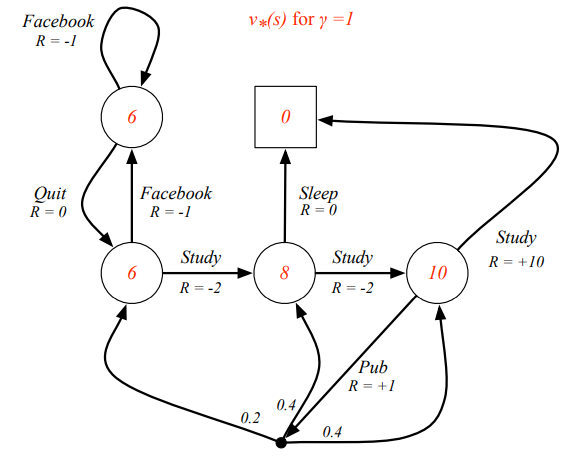yyxsb best state value

Also, via $(9)$, we can get action-state value: 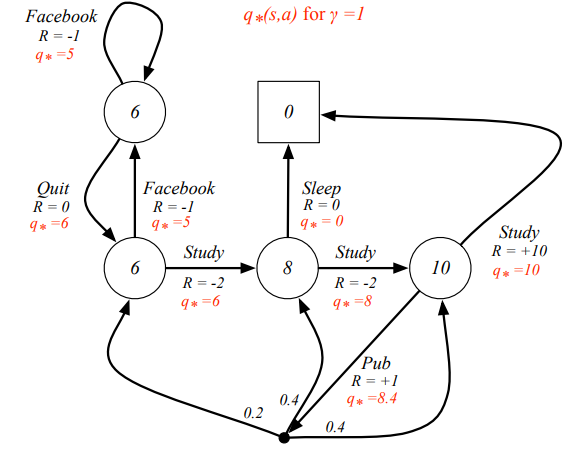yyxsb best state action value

But the question is: How to tell machine that policy $1$ is better than policy $2$? We need to define it clearly: $\pi \geq \pi^{\prime} \text { if } v_{\pi}(s) \geq v_{\pi^{\prime}}(s), \forall s$ Also very beautiful, right?
Theorem: For any MDP

• There exists an optimal policy $\pi_{*}$ that is better than or equal to all other policies, $\pi_{*} \geq \pi, \forall \pi$
• All optimal policies achieve the optimal value function, $v_{\pi_{*}}(s) = v_{*}(s)$
• All optimal policies achieve the optimal action-value function, $q_{\pi_{*}}(s, a) = q_{*}(s,a)$

We don’t prove this theorem here because it doesn’t affect our understanding, just believe it!

Finally, I will show you how to find an optimal policy!

An optimal policy can be found by maximising over $q$ $\pi_{*}(a | s)=\left\{\begin{array}{ll}{1} & {\text { if } a=\underset{a \in \mathcal{A}}{\operatorname{argmax}} q_{*}(s, a)} \\ {0} & {\text { otherwise }}\end{array}\right.$

• There is always a deterministic optimal policy for any MDP
• If we know $q_{*}(s, a)$, we immediately have the optimal policy

Let’s check the theorem: 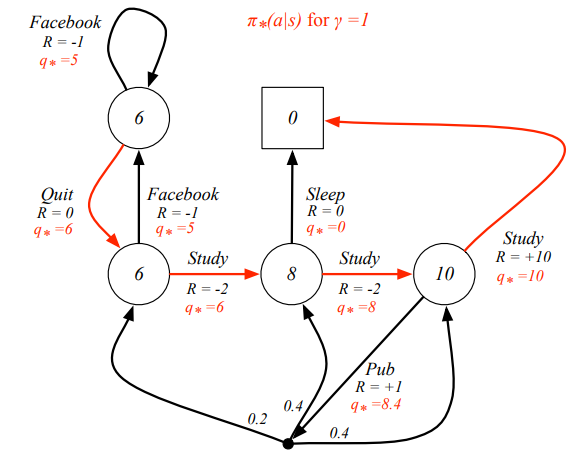yyxsb best policy

The next question is: how to calculate optimal state value or state action value via math equations? $v_{*}(s)=\max _{a} q_{*}(s, a)$ $q_{*}(s, a)=\mathcal{R}_{s}^{a}+\gamma \sum_{s^{\prime} \in \mathcal{S}} \mathcal{P}_{s s^{\prime}}^{a} v_{*}\left(s^{\prime}\right)$ $v_{*}(s)=\max _{a} \mathcal{R}_{s}^{a}+\gamma \sum_{s^{\prime} \in \mathcal{S}} \mathcal{P}_{s s^{\prime}}^{a} v_{*}\left(s^{\prime}\right)$ $q_{*}(s, a)=\mathcal{R}_{s}^{a}+\gamma \sum_{s^{\prime} \in \mathcal{S}} \mathcal{P}_{s s^{\prime}}^{a} \max _{a^{\prime}} q_{*}\left(s^{\prime}, a^{\prime}\right)$

Programming these guys are not so easy, but you can try it yourself.
About how to find (sub)optimal policy $\pi$ through computer programs, I will show you in other posts.

Summary

In this post, I’ve showed you how to understand MDP easily through many examples and codes. Understanding MDP is the key point in mastering reinforcement learning. How to get policy in computer programs are not been described and please check for this post: An Easy Way To Understand Markov Decision Process In Reinforcement Learning.

References

• David Silver-Markov Decision Processes
• Reinforcement Learning and Markov Decision Processes
• Getting Started with Markov Decision Processes: Reinforcement Learning
• Pythonではじめる強化学習
• Bellman equations and optimal policies

---

You May Also Enjoy

A Least Squares Approach --Math

Linear Modeling - A Maximum Likelihood Approach --Math

The Bayesian Approach To Machine Learning --Math

An Introduction To ESN --Math

Modeling With NMF And SVD --Math

Bounding Box Regression --Math

Welcome to share or comment on this post: